This is a ‘living’ glossary for the Oracle Optimizer I’ve put together for quick reference. It’s derived from the glossary in the SQL Tuning Guide with some additions and extra links.
I’ve broken it up into the following sections:
- Optimizer Features
- Costing and Optimization
- Execution Plans
- Optimizer Statistics
- Plan Management
- Join Types and Join Methods
- Transformations and Expansions
- Optimizing Data Processing and Access
- General Terminology
Optimizer Features
Adaptive Cursor Sharing (ACS)
ACS allows the Oracle Database to generate multiple execution plans for a single SQL statement using bind variables, based on the runtime bind values and their selectivity.
Cursor states:
- Bind-insensitive: The plan is good for all bind values.
- Bind-sensitive: Oracle starts monitoring behavior with different bind values.
- Bind-aware: Oracle creates and uses different plans based on observed bind value selectivity.
The performance view V$SQL has columns IS_BIND_AWARE and IS_BIND_SENSITIVE for viewing cursor states associated with ACS.
Example:
SELECT * FROM orders WHERE customer_id = :b1;
If “:b1” is often a very selective value (few rows) but sometimes not (many rows), ACS can keep both a “selective” plan (index access) and a “non-selective” plan (full scan).
Useful view: V$SQL, columns IS_BIND_AWARE and IS_BIND_SENSITIVE
More info:
Adaptive Dynamic Sampling
A feature of the adaptive optimizer that enables the automatic adjustment of the dynamic statistics level. It is associated with optimizer adaptive statistics and dynamic sampling level 11 (set using the OPTIMIZER_DYNAMIC_SAMPLING database parameter).
More info:
Adaptive Plans
Adaptive plans (or optimizer adaptive plans) enable the optimizer to make a plan decision for a SQL statement after parsing has completed and during execution. This enables the optimizer to correct some classes of problems at runtime:
- Join method: hash vs nested loops
- Use of bitmap indexes
- Parallel distribution methods
Adaptive plans are enabled by default using the database parameter OPTIMIZER_ADAPTIVE_PLANS.
See also: adaptive query plan
More info:
Adaptive Statistics
Adaptive statistics (or optimizer adaptive statistics) are a set of capabilities within the adaptive query optimisation framework that allow the optimizer to make run-time adjustments to execution plans and discover additional information that can lead to better statistics.
The feature makes use of SQL plan directives, statistics feedback, and adaptive dynamic sampling.
The capability is controlled by the optimizer_adaptive_statistics database parameter and is disabled by default in Oracle Database 12c Release 2 and onwards using the database parameter OPTIMIZER_ADAPTIVE_STATISTICS.
More info:
Bind-aware Cursor
A bind-sensitive cursor that is eligible to use different plans for different bind values. After a cursor has been made bind-aware, the optimizer chooses plans for future executions based on the bind value and its cardinality estimate.
Example:
SELECT * FROM sales WHERE region_id = :r;
After several executions with varying selectivity for the values of “:r”, the cursor becomes bind-aware and, for small regions, uses an index access plan for the region_id column and, for large regions, uses a full table scan to access the SALES table.
See also Adaptive Cursor Sharing.
Bind-insensitive Cursor
A cursor whose optimal plan does not depend on the value of bind variables.
Example:
SELECT COUNT(*) FROM big_table WHERE status = :s;
If an index is never beneficial for any value of “:s”, one plan (full scan) suffices.
See also Adaptive Cursor Sharing.
Bind-sensitive Cursor
A cursor whose optimal plan may depend on the value of a bind variable. The database monitors the behavior of a bind-sensitive cursor that uses different bind values to determine whether a different plan is beneficial. A bind-sensitive cursor may become bind-aware after a few executions.
Example:
SELECT * FROM accounts WHERE acct_type = :t;
Different selectivities for the value of “:t” lead Oracle to monitor and possibly create separate plans.
See also Adaptive Cursor Sharing.
Bind Variable Peeking
The ability of the optimizer to look at the value in a bind variable during a hard parse. By peeking at bind values, the optimizer can determine the selectivity of a WHERE clause condition as if literals had been used, thereby improving the plan. It works in concert with adaptive cursor sharing.
Example:
SELECT * FROM customers WHERE cust_type = :b;
First execution sees :b = ‘VIP’, very selective, yielding an index plan. Later executions with non-selective values may prompt ACS to add a second plan.
See also Adaptive Cursor Sharing.
Cardinality Feedback
See statistics feedback.
Cost-Based Optimization
The primary optimization approach used by the Oracle Database. It is a strategy for choosing the most efficient execution plan for a SQL statement, largely based on optimizer statistics and estimated cost.
Example:
- For a join of orders and customers, the optimizer weighs nested loops with index vs. hash join with full scans based on row counts and costs.
More info:
Cost-based Optimizer (CBO)
The legacy name for the Oracle Optimizer. In earlier releases, the cost-based optimizer was an alternative to the rule-based optimizer (RBO). The CBO calculates the “cost” of various execution plans and chooses the one with the lowest cost. The cost is a relative measure based on estimated resource consumption (CPU, I/O).
Dynamic Sampling
Dynamic sampling, also referred to as dynamic statistics in Oracle Database 12c Release 1 (12.1) and later releases, is an optimisation technique where the database executes an internal SQL statement to scan a small random sample of a table’s blocks to estimate predicate selectivities, thus leading to more accurate cardinality estimates.
Dynamic Statistics
An optimization technique in which the database executes an internal (recursive) SQL statement to scan a small random sample of a table’s blocks to estimate predicate selectivities, thus leading to more accurate cardinality estimates.
More info:
Dynamic Statistics Level
The level that controls both when the database gathers dynamic statistics, and the size of the sample that the optimizer uses to gather the statistics. Set the dynamic statistics level using either the OPTIMIZER_DYNAMIC_SAMPLING initialization parameter or a statement hint (DYNAMIC_SAMPLING).
More info:
Hint
Directives embedded within a SQL statement that allow developers to influence the optimizer’s choices. While powerful, they should be used judiciously as they can override optimal behavior if not carefully considered.
Examples:
/*+ USE_INDEX(table_name index_name) *//*+ FULL(table_name) */
More info:
Logical Optimizer
The logical optimizer is part of the overall Oracle Optimizer.
The logical optimizer (also known as the query transformation phase) focuses on restructuring the SQL query to produce a logically equivalent query that might be more efficient to execute.
See also physical optimizer.
More info:
Optimization
The overall process of choosing the most efficient means of executing a SQL statement.
Optimizer
Built-in database software that determines the most efficient way to execute a SQL statement by considering factors related to the objects referenced and the conditions specified in the statement.
Outline
A special type of optimizer hint that fully specifies an execution plan. Outline hints are used internally by Oracle to recreate a specific execution plan.
You can see a SQL statements’ outline using the “OUTLINE” keyword in DBMS_XPLAN format. For example:
SELECT FROM TABLE(DBMS_XPLAN.DISPLAY_CURSOR(format=>'typical +outline'));
Performance Feedback
This form of automatic re-optimization helps improve the degree of parallelism automatically chosen for repeated SQL statements. It is enabled with automatic degree of parallelism and is therefore activated when PARALLEL_DEGREE_POLICY is set to ADAPTIVE.
Physical Optimizer
The physical optimizer is part of the overall Oracle Optimizer.
The physical optimizer takes the transformed (logical) query and determines the best execution plan based on statistics, access paths, and available operations.
See also logical optimizer.
Pipelined Table Function
A PL/SQL function that returns multiple rows, one at a time or in batches. It can be invoked if used as an operand of the TABLE operator in the FROM list of a SELECT statement.
Example:
SELECT * FROM TABLE(stream_orders_fn(:batch_id));
Rows “stream” to the caller as they are produced.
Plan Generator
The part of the optimizer that tries different access paths, join methods, and join orders for a given query block to find the plan with the lowest cost.
Recursive SQL
Additional SQL statements that the database must issue to execute a SQL statement issued by a user. The generation of recursive SQL is known as a recursive call. For example, the database generates recursive calls when data dictionary information is not available in memory and so must be retrieved from disk.
SQL Plan Directive
Additional information and instructions that the optimizer can use to generate a more optimal plan. For example, a SQL plan directive might instruct the optimizer to collect missing statistics or gather dynamic statistics. They are visible in the DBA_SQL_PLAN_DIRECTIVES view.
The optimizer uses SQL plan directives if OPTIMIZER_ADAPTIVE_STATISTICS is set to the non-default value TRUE.
More info:
Statistics Feedback
Previously known as cardinality feedback.
A form of automatic re-optimization that automatically re-parses SQL to improve execution plans that have cardinality misestimates. The optimizer may estimate cardinalities incorrectly, particularly if a query has many complex predicates. Statistics feedback aims to address this by re-parsing and improving cardinality estimates iteratively. This allows the optimizer to react to inaccuracies in initial estimates.
The performance view V$SQL includes a column called IS_REOPTIMIZABLE to indicate the status of re-optimization. The view V$SQL_REOPTIMIZATION_HINTS contains additional information pertinent to the re-optimization process.
Costing and Optimization
Base Cardinality
For a table, base cardinality is the total number of rows in the table before any predicate filtering.
Example:
- If an EMPLOYEES table has 100,000 rows, its base cardinality is 100,000.
Cardinality
The estimated number of rows that a particular operation (e.g., a filter, a join) will return. Accurate cardinality estimates are crucial for the optimizer to choose an optimal plan. In the explain plan below, the cardinality of all operations is 105.
---------------------------------------------------------------------------------
| Id  | Operation           | Name      | Rows  | Bytes | Cost  | Pstart| Pstop |
---------------------------------------------------------------------------------
|   0 | SELECT STATEMENT    |           |   105 | 13965 |     2 |       |       |
|   1 |  PARTITION RANGE ALL|           |   105 | 13965 |     2 |     1 |     5 |
|   2 |   TABLE ACCESS FULL | EMP_RANGE |   105 | 13965 |     2 |     1 |     5 |
---------------------------------------------------------------------------------
More info:
Cost
A numeric internal measure that represents the estimated resource usage for an execution plan. The lower the cost, the more efficient the plan. In the explain plan below, the total cost of the SELECT statement (the line with Id = 0) is 2.
---------------------------------------------------------------------------------
| Id  | Operation           | Name      | Rows  | Bytes | Cost  | Pstart| Pstop |
---------------------------------------------------------------------------------
|   0 | SELECT STATEMENT    |           |   105 | 13965 |     2 |       |       |
|   1 |  PARTITION RANGE ALL|           |   105 | 13965 |     2 |     1 |     5 |
|   2 |   TABLE ACCESS FULL | EMP_RANGE |   105 | 13965 |     2 |     1 |     5 |
---------------------------------------------------------------------------------
Cost is a relative unit, not a literal CPU or I/O count. Costs across statements are not directly comparable without the same optimizer environment.
More info:
Cost Model
The mathematical model used by the optimizer to calculate the cost of an execution plan. It considers factors like I/O operations and CPU usage.
Density
A decimal number between 0 and 1 that measures the selectivity of a column. Values close to 1 indicate that the column is unselective, whereas values close to 0 indicate that this column is more selective.
For example, consider a table (TAB1) and a column (COL1) containing values 1 to 10 (with no NULL values). The density of COL1 is 1/10, which equals 0.1.
Estimator
The component of the optimizer that determines the overall cost of a given execution plan.
Expected Cardinality
For a table, the optimizer’s estimated number of rows the table has after all filter predicates have been applied.
Heuristic
A heuristic is a rule-based decision used by the optimizer to guide query optimization. The optimizer uses both heuristics and cost-based decisions to generate execution plans. Heuristics are generally applied before cost-based decisions are made.
Index Clustering Factor
A measure of row order in relation to an indexed value, such as employee last name. The more scattered the rows among the data blocks, the higher the clustering factor. When retrieving multiple rows from a table using an index, a low clustering factor means that fewer blocks from the table need to be visited to retrieve table column values than if the clustering factor is high.
Optimizer Environment
The totality of session settings that can affect execution plan generation, such as the work area size or optimizer settings (for example, the optimizer mode).
Example:
- ALTER SESSION SET optimizer_mode=first_rows(10); can change which join methods or access paths are chosen.
More info:
Optimizer Goal
The prioritization of resource usage by the optimizer. The OPTIMIZER_MODE initialization parameter can be used to set the goal ‘best throughput’ or ‘best response time’.
- ALL_ROWS: Optimizes for the best throughput, aiming to retrieve all rows as quickly as possible. This is the default.
- FIRST_ROWS and FIRST_ROWS(n): Optimizes for the best response time, aiming to retrieve the first ‘n’ rows as quickly as possible.
Selectivity
Selectivity refers to the fraction (or percentage) of rows from a table that are expected to match a query predicate (e.g., a WHERE clause condition).
For example:
SELECT * FROM employees WHERE dept_id= 10;
- Suppose there are 1000 employees, and 100 are in department 10
- Selectivity = 100 / 1000 = 0.1 (10%)
A formula for selectivity is:
selectivity = rows returned / base cardinality
Unselective
An informal term used when a relatively large fraction of rows are returned from a row set. A query becomes more unselective as the selectivity approaches 1.
For example, a query that returns 999,999 rows from a table with one million rows is unselective. A query of the same table that returns one row is selective.
Execution Plans
Accepted Plan
In the context of SQL plan management, a plan that is in a SQL plan baseline for a SQL statement and, thus, available for use by the optimizer.
More info:
Access Path
In the context of a SQL statement, it is how the database retrieves data from a database. For example, a query using an index and a query using a full table scan use different access paths.
More info:
Adaptive Plan
See adaptive query plan.
Adaptive Query Plan
An execution plan that changes after optimization because run-time conditions indicate that optimizer estimates are inaccurate. An adaptive query plan has different built-in plan options. During the first execution, before a specific subplan becomes active, the optimizer makes a final decision about which option to use. The optimizer bases its choice on observations made during the execution up to this point. Thus, an adaptive query plan enables the final plan for a statement to differ from the default plan.
More info:
Common Table Expressions (CTEs)
See subquery factoring.
Condition
A combination of one or more expressions and logical operators that returns a value of TRUE, FALSE, or UNKNOWN.
Correlated Subquery
A type of subquery that depends on values from the outer query. Unlike a regular (non-correlated) subquery, it cannot be run independently because it refers to a column from the outer query’s row.
Example:
SELECT e.*FROM emp eWHERE e.salary >
(SELECT AVG(salary) FROM emp WHERE deptno = e.deptno);
Cursor-duration Temporary Table
A temporary table instantiated during query execution that stores query results for the duration of a cursor. For complex operations such as WITH clause queries and star transformations, this optimization enhances the materialization of intermediate results from repetitively used subqueries. In this way, cursor-duration temporary tables improve performance and optimizes I/O.
Example:
- A complex WITH query executed multiple times within a statement may be materialized into a cursor-duration temporary table to avoid recomputation.
Default Plan
For an adaptive query plan, it is the execution plan initially chosen by the optimizer using the statistics from the data dictionary. The default plan can differ from the final plan.
Dynamic Plan
If an adaptive query plan is deemed appropriate during optimization, multiple subplans may be chosen for a query. The final subplan used at run time depends on the statistics obtained by the optimizer statistics collector.
Execution Plan
The combination of steps used by the database to execute a SQL statement. Each step either retrieves rows of data physically from the database or prepares them for the session issuing the statement. It defines the order of operations, access paths, join methods, and other details. It is typically viewed using DBMS_XPLAN or SQL Monitor.
Execution Tree
A tree diagram that shows the flow of row sources from one step to another in an execution plan.
Explain Plan
A SQL utility (EXPLAIN PLAN FOR statement) that displays the execution plan for a given SQL statement without actually executing it.
Example:
EXPLAIN PLAN FOR SELECT * FROM emp WHERE empno = 10;
SELECT * FROM TABLE(DBMS_XPLAN.DISPLAY);
More info:
Expression
A combination of one or more values, operators, and SQL functions that evaluates to a value. For example, the expression 2*2 evaluates to 4. In general, expressions assume the data type of their components.
More info:
Filter Condition
A WHERE clause component that eliminates rows from a single object referenced in a SQL statement.
Example:
WHERE hire_date >= DATE '2024-01-01'
Final Plan
In an adaptive plan, the plan that executes to completion. The default plan can differ from the final plan.
Inline View
An inline view is a subquery that is placed within the FROM clause of a SELECT statement. It effectively creates a temporary, named result set that the outer query can then treat as a table. Inline views can also be created using the WITH clause, which can enhance readability and maintenance in complex queries.
Example:
SELECT *
FROM (
    SELECT deptno, AVG(sal) avg_sal
    FROM emp
    GROUP BY deptno) v
WHERE v.avg_sal > 10000;
Non-correlated Subquery
Partition Pruning
An optimization technique where the database automatically eliminates unnecessary partitions from a query’s execution plan. For example, accessing specific index segments or scanning relevant partitions based on a query’s filter conditions.
Static partition pruning can occur at parse time if the relevant partition or partitions can be determined during optimization. Otherwise, dynamic pruning is where specific partitions are identified at run time.
Example:
WHERE order_date BETWEEN DATE '2025-01-01' AND DATE '2025-01-31'
On a monthly range-partitioned table, the database scans only the January 2025 partition.
See also partitioned table.
More info:
Predicate
A condition used to filter rows in a WHERE, JOIN, or HAVING clause.
Examples:
- t1.cust_id = t2.cust_id (join predicate)
- amount > 1000 (filter predicate)
Private Temporary Table
A memory-only temporary table whose data and metadata is session-private.
Query Block
A top-level SELECT statement, a subquery, or an unmerged view
Subplan
A portion of an adaptive plan that the optimizer can switch to as an alternative at run time. A subplan can consist of multiple operations in the plan. For example, the optimizer can treat a join method and the corresponding access path as one unit when determining whether to change the plan at run time.
Subplan Group
A set of subplans in an adaptive query plan.
Subquery
A query nested within another SQL statement.
See also correlated subquery.
Example:
SELECT *
FROM emp
WHERE deptno IN
    (SELECT deptno FROM dept WHERE location = 'BOSTON');
Subquery Factoring
Subquery factoring clauses are synonymous with WITH clauses in SQL statements. They are used to logically break up and simplify complex queries to make them reusable and easier to read.
Example:
WITH high_sal AS
   (SELECT empno FROM emp WHERE sal > 10000)
SELECT *
FROM emp e JOIN high_sal h ON e.empno = h.empno;
Uncorrelated Subquery
A type of subquery that does not depend on values from the outer query.
See also correlated subquery.
Example:
SELECT * FROM emp WHERE sal > (SELECT AVG(sal) FROM emp);
Optimizer Statistics
Column Group
A set of two or more columns for which Oracle maintains combined statistics to better estimate row counts (cardinality) and selectivity during query optimization.
For example:
BEGIN
  DBMS_STATS.CREATE_EXTENDED_STATS(
    ownname => 'HR',
    tabname => 'EMPLOYEES',
    extension => '(DEPARTMENT_ID, JOB_ID)'
  );
END;
/
The data dictionary view ALL_STAT_EXTENSIONS exposes column groups.
See also extended statistics.
More info:
Column Statistics
Statistics about columns that the optimizer uses to determine optimal execution plans. Column statistics include the number of distinct column values, low value, high value, and number of nulls. They can be viewed in the ALL_TAB_COL_STATISTICS dictionary view.
Data Skew
Large variations in the data distribution of values in a column.
- Range skew refers to a non-uniform distribution of data values across a column’s range. For example, a column may have a range of values from 1 to 1000, but could be missing values between 500 and 900. That would constitute range skew.
- Value skew refers to the uneven frequency of specific values within a column. For example, a column may contain values 1 to 2, but one row with value 1 and 1000 rows with value 2. That would constitute value skew.
Histograms are used to characterize range and value skew.
More info:
Endpoint Number
A number that uniquely identifies a bucket in a histogram. In frequency and hybrid histograms, the endpoint number is the cumulative frequency of endpoints. In height-balanced histograms, the endpoint number is the bucket number.
More info:
Endpoint Repeat Count
In a hybrid histogram, the number of times the endpoint value is repeated for each endpoint (bucket) in the histogram. By using the repeat count, the optimizer can obtain accurate estimates for popular values.
More info:
Endpoint Value
An endpoint value is the highest value in the range of values in a histogram bucket.
More info:
Expression Statistics
A type of extended statistics that improves optimizer estimates when a WHERE clause has predicates that use expressions.
Extended Statistics
A type of optimizer statistic that improves estimates for cardinality when multiple predicates exist or when predicates contain an expression.
More info:
Extension
A column group or an expression statistics.
Extensions cover both column groups and expression statistics, created with DBMS_STATS.CREATE_EXTENDED_STATS.
The statistics collected for column groups and expressions are called extended statistics.
Fixed Object Statistics
Fixed object statistics are optimizer statistics gathered on fixed objects, which are dynamic performance tables and their associated indexes. These objects record current database activity and are owned by the user SYS. They can be gathered with DBMS_STATS.GATHER_FIXED_OBJECT_STATS.
Frequency Histogram
A type of histogram in which each distinct column value corresponds to a single bucket. An analogy is sorting coins: all pennies go in bucket 1, all nickels go in bucket 2, and so on.
More info:
Height-balanced Histogram
A histogram in which column values are divided into buckets so that each bucket contains approximately the same number of rows.
More info:
Histogram
A special type of column statistic that provides more detailed information about the data distribution in a table column.
Histograms help the optimizer make more accurate cardinality estimates when column values are not uniformly distributed.
More info:
Hybrid Histogram
An enhanced height-based histogram that stores the exact frequency of each endpoint in the sample, and ensures that a value is never stored in multiple buckets.
More info:
Incremental Statistics Maintenance
The ability of the database to generate global statistics for a partitioned table by aggregating partition-level statistics.
See also partitioned table.
More info:
Index Statistics
Statistics about indexes that the optimizer uses to determine whether to perform a full table scan or an index scan. Index statistics include B-tree levels, leaf block counts, the index clustering factor, distinct keys, and number of rows in the index. They can be seen in ALL_IND_STATISTICS.
Number of Distinct Values (NDV)
Count of unique values in a column. The NDV is important in generating cardinality estimates.
Non-popular Value
In a histogram, any value that does not span two or more endpoints. Any value that is not non-popular is a popular value.
More info:
Noworkload Statistics
Optimizer system statistics gathered when the database simulates a workload.
Workload system statistics are gathered while observing actual database workloads.
Example:
EXEC DBMS_STATS.GATHER_SYSTEM_STATS('NOWORKLOAD')
Optimizer Statistics
Statistics details about the database object used by the optimizer to select the best execution plan for each SQL statement. Categories include table statistics such as numbers of rows, index statistics such as B-tree levels, system statistics such as CPU and I/O performance, and column statistics such as number of nulls.
Metadata about the data in tables and indexes, including the number of rows, number of distinct values, average row length, and data distribution (histograms). Accurate and up-to-date statistics are critical for the CBO.
More info:
Optimizer Statistics Advisor
A tool that inspects statistics gathering practices, automatically diagnoses problems with these practices, and generates a report of findings and recommendations.
More info:
Optimizer Statistics Advisor Rules
System-supplied standards by which Optimizer Statistics Advisor performs its checks.
Optimizer Statistics Collection
Optimizer statistics collection or gathering is the process of compiling statistics information on database objects. The database can collect these statistics automatically, or you can collect them manually by using the system-supplied DBMS_STATS package.
More info:
Optimizer Statistics Collector
A row source inserted into an execution plan at key points to collect run-time statistics for use in adaptive plans. A statistics collector is only used if adaptive plans are enabled.
See also adaptive plans.
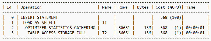
Optimizer Statistics Gathering
A plan operation used to gather optimizer statistics online during a bulk data load.
Example:
insert /*+ append */ into t1 select * from t2;
More info:
Optimizer Statistics Preferences
The default values of the parameters used by automatic statistics collection and the DBMS_STATS statistics gathering procedures.
More info:
Pending Statistics
Unpublished optimizer statistics. By default, the optimizer uses published statistics but does not use pending statistics.
Example:
- Gather with PUBLISH set to FALSE
- test in session with ALTER SESSION SET optimizer_use_pending_statistics=TRUE;
Popular Value
In a histogram, any value that spans two or more endpoints. Any value that is not popular is a non-popular value.
More info:
Real-time Statistics
Supplemental statistics collected automatically during conventional DML operations. Note that they do not replace the need for gathered optimizer statistics.
More info:
Synopsis
A set of auxiliary statistics gathered on a partitioned table when the INCREMENTAL value is set to true.
See also partitioned table and incremental statistics.
System Statistics
Statistics that enable the optimizer to use CPU and I/O characteristics. They are used by the cost model to adjust cost calculations.
More info:
Table Statistics
Statistics about tables that the optimizer uses to determine table access cost, join cardinality, join order, and so on. Table statistics include row counts, block counts, empty blocks, average free space per block, number of chained rows, average row length, and staleness of the statistics on the table. They can be seen in the ALL_TAB_STATISTICS dictionary view.
Top Frequency Histogram
A variation of a frequency histogram that ignores non-popular values that are statistically insignificant, thus producing a better histogram for popular values
More info:
Plan Management
Automatic Capture Filter
A SQL plan management feature that enables you to specify the eligibility criteria for automatic initial plan capture using DBMS_SPM.CONFIGURE. Used in conjunction with the database initialization parameter optimizer_capture_sql_plan_baselines.
More info:
Automatic Initial Plan Capture
The mechanism by which the database automatically creates a SQL plan baseline for any repeatable SQL statement executed on the database. Enable automatic initial plan capture by setting the optimizer_capture_sql_plan_baselines initialization parameter to true (the default is false).
Automatic SQL Plan Management
A feature that allows the Oracle database to capture SQL plan baselines automatically to prevent SQL plan performance regressions. Plan performance verification can be performed using a background task or in the foreground using real-time SPM.
More info:
Automatic SQL Tuning Set
The automatic SQL tuning set (ASTS or Auto STS) is a system-maintained SQL tuning set called SYS_AUTO_STS. It is used to capture workload SQL statements to support automatic features such as automatic indexing and automatic SQL plan management.
More info:
Disabled Plan
In the context of SQL plan management, a plan that a database administrator has manually marked as ineligible for use by the optimizer.
Example:
BEGIN
DBMS_SPM.ALTER_SQL_PLAN_BASELINE(..., attribute_name=>'ENABLED',
attribute_value=>'NO')
END;
/
Enabled Plan
In SQL plan management, a plan that is eligible for use by the optimizer.
Fixed Plan
An accepted plan that is marked as preferred, so that the optimizer considers only the fixed plans in the SQL plan baseline. You can use fixed plans to influence the plan selection process of the optimizer.
DBMS_SPM.ALTER_SQL_PLAN_BASELINE is used to fix a plan.
Manual Plan Capture
The user-initiated load of existing plans into a SQL plan baseline, such as:exec DBMS_SPM.LOAD_PLANS_FROM_CURSOR_CACHE
Plan Evolution
The change of an unaccepted plan in the SQL plan history into an accepted plan in the SQL plan baseline.
More info:
Plan Selection
The attempt to find a matching plan in the SQL plan baseline for a statement after performing a hard parse. If no plan baseline matches, the optimizer uses the plan chosen by the optimizer.
Plan Stability
Ensuring that a SQL statement consistently uses the same execution plan (or an ‘approved’ execution plan) over time, even with changes in data or environment.
Plan Verification
Comparing the performance of an unaccepted plan to a plan in a SQL plan baseline.
Real-time SQL plan management
A subcomponent of automatic SQL plan management. It allows the Oracle database to capture SQL plan baselines automatically to prevent SQL plan performance regressions. Plan performance verification is performed in the foreground (client) process rather than in the background.
More info:
Repeatable SQL Statement
A repeatable SQL statement is one where its SQL signature does not change (i.e. the SQL text remains the same while making allowances for differences in white space and case), and the database hard parses more than once. SQL statements are tracked in the SQL statement log to monitor repeatability.
Example:
SELECT * FROM sales WHERE sale_id = :bind1;
SQL Handle
A string value derived from the numeric SQL signature. Like the signature, the handle uniquely identifies a SQL statement. It serves as a SQL search key in user APIs. SQL handles can be viewed in DBA_SQL_PLAN_BASELINES.
SQL Management Base (SMB)
A logical repository that stores statement logs, plan histories, SQL plan baselines, and SQL profiles. The SMB is part of the data dictionary and resides in the SYSAUX tablespace.
SQL Management Object (SMO)
A feature that stabilizes the execution plans of individual SQL statements. Examples include SQL profiles, SQL plan baselines, and SQL patches.
SQL Patch
A SQL Patch is a SQL management object that is used to change or fix the behavior of a SQL statement.
More info:
SQL Plan History
A SQL execution plan captured by SQL plan management but has not been ‘accepted’ (and thus added to the SQL plan baseline). It can be thought of as an ‘unaccepted SQL plan baseline’. They appear in the view DBA_SQL_PLAN_BASELINES where the ACCEPTED column has the value NO.
More info:
SQL Plan Baseline
A set of one or more accepted plans for a repeatable SQL statement. Plan baselines allow the optimizer to capture known execution plans for a SQL statement and specify which plans can be used. In general, only “accepted” plans in the baseline can be used, ensuring plan stability and preventing regressed performance. Unaccepted plans listed in the database view DBA_SQL_PLAN_BASELINES are part of the SQL plan history rather than the SQL plan baseline.
More info:
SQL Plan Capture
Techniques for capturing and storing relevant information about plans in the SQL management base (SMB) for a set of SQL statements. Capturing a plan means making SQL plan management aware of this plan.
More info:
SQL Plan Management (SPM)
SQL plan management is a mechanism that records and evaluates the execution plans of SQL statements over time. SQL plan management can prevent SQL plan regressions caused by environmental changes such as a new optimizer version, changes to optimizer statistics, system settings, and so on.
The key features and components are:
- SQL Plan Baseline: a set of one or more accepted execution plans for a specific SQL statement. Only these plans are eligible for use by the optimizer.
- Plan Capture: the process of recording execution plans from the cursor cache or SQL tuning sets. Can be automatic or manual.
- Plan Selection: the optimizer uses only enabled and accepted plans from the baseline. If no baseline exists, it proceeds with normal cost-based optimization.
- Plan Evolution: the process of evaluating new plans and accepting them into the baseline only if they perform better. Evolution can be achieved automatically or manually.
More info:
SQL Profile
A SQL management object create by the SQL Tuning Advisor that helps the optimizer generate better execution plans. It provides additional statistics and corrections that help the optimizer make better decisions.
SQL Signature
A numeric hash value computed using a SQL statement text that has been normalized for case insensitivity and white space. It uniquely identifies a SQL statement. The database uses this signature as a key to maintain SQL management objects such as SQL profiles, SQL plan baselines, and SQL patches. For example, the DBA_SQL_PLAN_BASELINES view includes a SIGNATURE column.
SQL Statement Log
When automatic SQL plan capture is enabled, a log that contains the SQL ID of SQL statements that the optimizer has evaluated over time. A statement is tracked when it exists in the log.
SQL Tuning Advisor
An automated tool that analyzes SQL statements and provides tuning recommendations to improve their performance. It may recommend the creation of a SQL profile to improve a SQL execution plan.
More info:
Stored Outlines
A deprecated feature for storing hints associated with a SQL statement, superseded by SQL plan management. The hints in stored outlines direct the optimizer to choose a specific plan for the statement.
Unaccepted Plan
A plan for a statement that is in the SQL plan history but has not been added to the SQL plan baseline.
Join Types and Join Methods
Antijoin
A join type that returns rows that fail to match the subquery on the right side. For example, an antijoin can list departments with no employees. Antijoins use the NOT EXISTS or NOT IN constructs.
Example:
SELECT d.deptno
FROM  dept d
WHERE NOT EXISTS (
    SELECT 1 FROM emp e WHERE e.deptno = d.deptno);
Band Join
A special type of non-equijoin join type in which key values in one data set must fall within the specified range (“band”) of the second data set. Typically, they are used in time-range correlations.
Example:
WHERE e.event_ts BETWEEN w.start_ts AND w.end_ts;
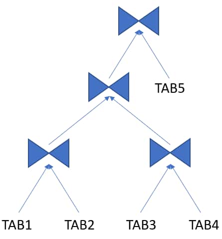
Bushy Join Tree
A join tree in which the left or the right child of an internal node can be a join node.
More info:
Cross Join
A join type that returns every combination of rows: a Cartesian join.
Example:
SELECT * FROM t1 CROSS JOIN t2;
Cartesian Join
A join type in which one or more of the tables does not have any join conditions to any other tables in the statement. The optimizer joins every row from one data source with every row from the other data source, creating the Cartesian product of the two sets.
- Joins every row of one table to every row of the other (no join condition).
- Typically used intentionally in special cases, but can otherwise indicate a missing join predicate in the SQL statement.
Example:
SELECT * FROM t1, t2;
Cartesian Product
A join type that returns every combination of rows from both tables in the join.
Driving Table
The table to which other tables are joined. An analogy from programming is a for loop that contains another for loop. The outer for loop is the analog of a driving table.
Equijoin
A join type whose join condition contains an equality operator.
Example:
SELECT t1.surname, t2.department_name
FROM   staff t1
JOIN departments t2 ON t1.deptno = t2.deptno;
Full Outer Join
A combination of a left and right outer join. In addition to the inner join, the database uses nulls to preserve rows from both tables that have not been returned in the result of the inner join. In other words, full outer joins join tables together, yet show rows with no corresponding rows in the joined tables.
Example:
SELECT … FROM t1 FULL OUTER JOIN t2 ON t1.id = t2.id;
Hash Join
A method for joining large data sets. The database uses the smaller of two data sets to build a hash table on the join key in memory. It then scans the larger data set, probing the hash table to find the joined rows.
Inner Join
A join type of two or more tables that returns only those rows that satisfy the join condition.
Inner Table
In a nested loops join, the table that is not the outer table (driving table). For every row in the outer table, the database accesses rows from the inner table.
Join
A statement that retrieves data from multiple tables specified in the FROM clause of a SQL statement. Join types include inner joins, outer joins, and Cartesian joins.
More info:
Join Condition
A condition that compares two row sources using an expression. The database combines rows from each row source, for which the join condition evaluates to true.
Example:
SELECT t1.name, t2.street_name
FROM   customers t1, addresses t2
WHER   t1.cust_id = t2.cust_id;
Join Group
A user-created database object that specifies a group of columns that participate in a join. Join groups are only supported in the In-Memory column store.
Join Method
A method of joining a pair of row sources. For example, nested loop, sort merge, and hash joins.
More info:
Join Tree
A join tree is also called a join graph or join order tree. It represents how multiple tables are joined together in a SQL query, and it implies a join order from the bottom to the top of the tree.
More info:
Join Type
The type of join specified in the SQL statement. For example, inner join, left outer join.
More info:
Join Order
The order in which multiple tables are joined together. For example, for each row in the employees table, the database can read each row in the departments table. In an alternative join order, for each row in the departments table, the database reads each row in the employees table.
To execute a statement that joins more than two tables, Oracle joins two of the tables and then joins the resulting row source to the next table. This process continues until all tables are joined into the result.
The order in which tables are joined can significantly affect performance, so the optimizer aims to find the most efficient one.
More info:
Join Predicate
A predicate in a WHERE or JOIN clause that combines the columns of two tables in a join.
Example:
SELECT t1.name, t2.street_name
FROM   customers t1, addresses t2
WHERE  t1.cust_id = t2.cust_id;
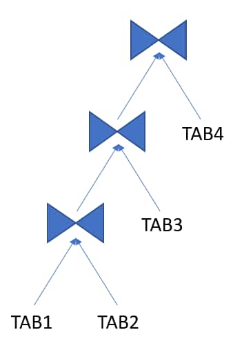
Left Deep Join Tree
A join tree in which the left input of every join is the result of a previous join (except for the first table, TAB1 in the example).
Example:
More info:
Left Outer Join
A join type that includes all rows from the left table and matched rows from the right.
Left Table
In an outer join, the table specified on the left side of the OUTER JOIN keywords (in ANSI SQL syntax). Appears on the left in a join tree.
Nested Loops Join
A type of join method, best for joining a small number of rows. A nested loops join determines the outer table that drives the join, and for every row in the outer table, probes each row in the inner table. The outer loop is for each row in the outer table and the inner loop is for each row in the inner table. An analogy from programming is a for loop inside of another for loop.
Non-equijoin
A join type whose join condition does not contain an equality operator.
Example:
SELECT t1.surname, t2.department_name
FROM   staff t1
JOIN departments t2 ON t1.deptno <> t2.deptno;
Non-join Column
A predicate in a WHERE clause that references only one table.
Outer Join
A join type using the outer join operator (+) or ANSI OUTER JOIN syntax with one or more columns of one of the tables. The database returns all rows that meet the join condition, along with unmatched rows padded with NULL values.
More info:
Outer Table
See driving table.
Partition-wise Join
A join optimization that divides a large join of two tables, one of which must be partitioned on the join key, into several smaller joins.
See also partitioned table.
More info:
Right Outer Join
A join type that includes all rows from the right table, matched rows from the left.
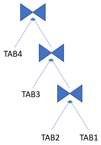
Right Deep Join Tree
A join tree in which the right input of every join is the result of a previous join (except for the first table, TAB1 in the example).
More info:
Right Table
Refers to the table that is on the right side of a join (and on the right in a join tree).
Self Join
A table joined to itself, usually with table aliases.
Example:
SELECT e.empno emp, m.empno manager
FROM   emp e JOIN emp m ON e.mgr = m.empno;
More info:
Semi Join
A type of join that returns rows from one table where a match exists in another table but does not return any columns from the second (matched) table. It optimizes subqueries with IN or EXISTS.
More info:
Sort Merge Join
A type of join method. The join consists of a sort join, in which both inputs are sorted on the join key, followed by a merge join, in which the sorted lists are merged.
More info:
Transformations and Expansions
Complex View Merging (CVM)
Complex View Merging (CVM) is a transformation where complex views are merged into the outer query, where, traditionally, they could not be merged (due to constructs like GROUP BY, DISTINCT, HAVING, etc.).
It extends regular view merging to support more sophisticated views, enabling more powerful optimization strategies.
More info:
Cost-based OR Expansion Transformation (CBOR)
Expands OR conditions into UNION ALL or multiple branches for better index use. The decision to use the transformation is cost-based, in contrast to the legacy OR transformation, which used heuristics.
Expansion
An expansion duplicates a portion of a query, typically in OR conditions or set operations (such as UNION ALL), to optimize each part separately and combine the results.
Group-by Placement
When possible, the optimizer repositions GROUP BY clauses for early aggregation. It can be advantageous to group rows as soon as possible in the execution plan, reducing the number of rows processed in subsequent joins.
Join Commutation/Associativity
Allows the optimizer to reorder joins by commuting (swapping the left and right inputs of a join) and associating (regrouping chains of joins) so it can evaluate more join orders and choose the lowest-cost one.
Join Conversion
Converts outer joins to inner joins (or vice versa) when safe and beneficial.
Join Elimination
The removal of redundant tables from a query. A table is redundant when its columns are only referenced in join predicates, and those joins are guaranteed to neither filter nor expand the resulting rows.
For example, when joining to a primary key of a foreign key table, where only the key is referenced, can be eliminated.
Join Factorization
A cost-based transformation that can factorize common computations from branches of a UNION ALL query. Without join factorization, the optimizer evaluates each branch of a UNION ALL query independently, which leads to repetitive processing, including data access and joins. Avoiding an extra scan of a large base table can lead to huge performance improvements.
Join Predicate Pushdown (JPPD)
Join Predicate Pushdown (JPPD) in Oracle is a cost-based query transformation where join conditions (or related predicates) are pushed into a subquery/view so Oracle can filter rows earlier, reduce intermediate row counts, and sometimes enable better access paths (e.g., index range scans, partition pruning).
Example:
SELECT o.order_id, o.order_date
FROM   orders o
JOIN   ( SELECT customer_id
         FROM   customers
         WHERE  region = 'US'
       ) c
ON     c.customer_id = o.customer_id
WHERE  o.status = 'SHIPPED';
Can be transformed to:
SELECT o.order_id, o.order_date
FROM   orders o
WHERE  o.status = 'SHIPPED'
AND    EXISTS (
         SELECT 1
         FROM   customers c
         WHERE  c.region = 'US'
         AND    c.customer_id = o.customer_id
       );
This helps when the inline view would otherwise return many rows (e.g., all US customers), but the driving table predicate (o.status=’SHIPPED’) is selective.
Predicate Pushing
A transformation technique in which the optimizer “pushes” the relevant predicates from the containing query block into the view query block. For views that are not merged, this technique improves the subplan of the unmerged view because the database can use the pushed-in predicates to access indexes or to use as filters.
More info:
Predicate Pushdown
Moving filter predicates as close to the data source as possible for performance.
More info:
Projection View
An optimizer-generated view that appears in queries in which a DISTINCT view has been merged, or a GROUP BY view is merged into an outer query block that also contains GROUP BY, HAVING, or aggregates.
Query rewrite
An optimizer feature that automatically transforms a user’s query into a different but semantically equivalent query, typically to improve performance using materialized views.
More info:
Simple View Merging
The merging of select-project-join views. For example, a query joins the employees table to a subquery that joins the departments and locations tables.
More info:
Star Transformation
Rewrites star-schema joins to bitmap index-based filtering for performance. It requires bitmap indexes on dimension keys, and the database star_transformation_enabled must be set to TRUE.
More info:
Subquery Unnesting
A transformation technique in which the optimizer transforms a nested query into an equivalent join statement, and then optimizes the join.
More info:
Table Expansion
A transformation technique that enables the optimizer to generate a plan that uses indexes on the read-mostly portion of a partitioned table, but not on the active portion of the table.
More info:
Transformation
The process by which the optimizer rewrites a SQL statement into an equivalent but more efficient form. Examples include view merging, subquery unnesting, and predicate pushdown.
More info:
Transitive Closure
A query transformation technique used by the optimizer to infer additional predicates based on existing ones.
For example, if A = B and B = C, then the optimizer can infer that A = C.
This inferred condition can then be used to optimize query performance, especially for join elimination, index usage, and partition pruning.
View Merging
The merging of a query block representing a view into the query block that contains it. View merging can improve plans by enabling the optimizer to consider additional join orders, access methods, and other transformations.
Merging a view into the main query allows the optimizer to treat the view as part of the outer query, enabling further optimizations.
More info:
View Subsumption
View subsumption is a heuristic query transformation technique that aims to improve query performance by reducing multiple table accesses and joins. It achieves this by unifying computations in multiple views into a single inline view (where possible and safe).
Optimizing Data Processing and Access
Access Path
The method used by the Oracle Optimizer to retrieve data from tables. Common access paths include full table scans, index scans (unique, range, skip), and cluster scans.
More info:
Bitmap Index
An index type optimized for columns with low cardinality.
More info:
Bitmap Join Index
A bitmap index for the join of two or more tables.
Bitmap Piece
A subcomponent of a single bitmap index entry. Each indexed column value may have one or more bitmap pieces. The database uses bitmap pieces to break up an index entry that is large in relation to the size of a block.
Approximate Query Processing
A set of optimization techniques that speed analytic queries by calculating results within an acceptable range of error.
More info:
Bloom Filter
A Bloom filter is a low-memory data structure used to test membership in a set. It can correctly indicate when an element is not in a set, but it may incorrectly indicate when an element is in a set; thus, false negatives are impossible, but false positives are possible. Bloom filters are particularly effective when the memory needed to store the filter is small relative to the data set size, and when most data is expected to fail the membership test.
More info:
B-tree Index
An index organized like an upside-down tree. A B-tree index has two types of blocks: branch blocks for searching and leaf blocks that store values. The leaf blocks contain every indexed data value and a corresponding rowid used to locate the actual row. The “B” stands for “balanced” because all leaf blocks automatically stay at the same depth.
More info:
Cluster Scan
An access path for a table cluster. In an indexed table cluster, Oracle Database first obtains the rowid of one of the selected rows by scanning the cluster index. Oracle Database then locates the rows based on this rowid.
Direct Path Read
A performance optimization where a single or multiblock read is processed directly in the program global area (PGA – an area of memory local to the client process). It bypasses the system global area (SGA) to improve the efficiency of processing the database blocks.
More info:
Foreign Key
A foreign key is a constraint that links two tables together by declaring or enforcing a relationship between a column (or group of columns) in one table and the primary key in another.
Full Table Scan
A scan of table data in which the database sequentially reads all rows from a table and filters out those that do not meet the selection criteria. All data blocks under the high water mark are scanned.
Used in cases where there is no usable index or where query predicates match a large proportion of rows in the table (or table partition).
More info:
Hash Cluster
A type of table cluster that is similar to an indexed cluster, except the index key is replaced with a hash function. No separate cluster index exists. In a hash cluster, the data is the index.
Hash Scan
An access path for a table cluster. The database uses a hash scan to locate rows in a hash cluster based on a hash value. In a hash cluster, all rows with the same hash value are stored in the same data block. To perform a hash scan, Oracle Database first obtains the hash value by applying a hash function to a cluster key value specified by the statement, and then scans the data blocks containing rows with that hash value.
More info:
Index
Optional schema object associated with a non-clustered table, table partition, or table cluster. In some cases indexes speed data access.
Indexes provide fast access to rows in a table based on the values in one or more columns. Oracle has B-tree, bitmap, and functional indexes.
Index Access Path
Data is retrieved from the database using an index to retrieve rows efficiently.
More info:
Index Cluster
A table cluster that uses an index to locate data. The cluster index is a B-tree index on the cluster key.
Index Fast Full Scan
A scan of the index blocks in unsorted order, as they exist on disk. This scan reads the index instead of the table.
More info:
Index Full Scan
The scan of an entire index in key order.
More info:
Index-organized Table
A table whose storage organization is a variant of a primary B-tree index. Unlike a heap-organized table, data is stored in primary key order.
Index Range Scan
Scanning an index for a range of values, commonly used for inequalities and ranges.
More info:
Index Range Scan Descending
An index range scan in which the database returns rows in descending order.
Index Skip Scan
An index scan occurs in which the initial column of a composite index is “skipped” or not specified in the query. For example, if the composite index key is (cust_gender,cust_email), then the query predicate does not reference the cust_gender column.
More info:
Index Unique Scan
A scan of an index that will return either zero or one rowid.
More info:
Multiblock Read
An I/O call that reads multiple database blocks. Multiblock reads can significantly speed up full table scans. For example, a data block might be 8 KB, but the operating system can read 1024 KB in a single I/O. For some queries, the optimizer may decide that it is more cost-efficient to read 128 data blocks in one I/O than in 128 sequential I/Os.
Parallel Execution
The application of multiple CPU and I/O resources to the execution of a single database operation.
More info:
Parallel Query
A query in which multiple processes work together simultaneously to run a single SQL query. By dividing the work among multiple processes, Oracle Database can run the statement more quickly. For example, four processes retrieve rows for four different quarters in a year instead of one process handling all four quarters by itself.
Running portions of the query simultaneously to improve performance.
More info:
Primary Key
A column or combination of columns that uniquely identifies each row in a table. In Oracle, uniqueness is enforced using unique indexes.
Table Cluster
A schema object that contains data from one or more tables, all of which have one or more columns in common. In table clusters, the database stores together all the rows from all tables that share the same cluster key.
Unique index
A unique index is a type of index that enforces uniqueness on the indexed column (or columns).
General Terminology
Bind Variable
A placeholder in a SQL statement that must be replaced with a valid value or value address for the statement to execute successfully. By using bind variables, you can write a SQL statement that accepts inputs or parameters at run time. The following query uses v_empid as a bind variable:
SELECT * FROM employees WHERE employee_id = :v_empid;
Child Cursor
The cursor containing the plan, compilation environment, and other information for a statement whose text is stored in a parent cursor. The parent cursor is number 0, the first child is number 1, and so on. Child cursors reference the same SQL text as the parent cursor but are different. For example, two queries with the text “SELECT * FROM t” use different cursors when they reference two different tables named “t”.
More info:
Cursor
A handle or name for a private SQL area in the program global area (PGA – a memory area local to the client process). Because cursors are closely associated with private SQL areas, the terms are sometimes used interchangeably.
See shared SQL area.
More info:
Cursor Cache
See shared SQL area.
Cursor Merging
Combining cursors to save space in the shared SQL area. It reduces child cursor proliferation when two child cursors share identical plans and metadata, thus reusing the same child.
Data Dictionary
A collection of tables and views that store metadata about the database, including information about tables, indexes, columns, and their statistics. The optimizer queries the data dictionary to gather information for plan generation.
Data Flow Operator (DFO)
The unit of work between data redistribution stages in a parallel query.
Degree of Parallelism (DOP)
The number of parallel execution servers associated with a single operation. Parallel execution is designed to effectively use multiple CPUs. Oracle Database parallel execution framework enables you to either explicitly choose a specific degree of parallelism or to rely on Oracle Database to automatically control it.
More info:
Dynamic Performance View
A view created on dynamic performance tables, which are virtual tables that record current database activity. The dynamic performance views are called fixed views because they cannot be altered or removed by the database administrator. They are also called V$ views because they begin with the string V$ (and GV$ in Oracle Real Application Clusters).
More info:
Extensible Optimizer
An optimizer capability that enables authors of user-defined functions and indexes to create statistics collection, selectivity, and cost functions that the optimizer uses when choosing an execution plan. The optimizer cost model is extended to integrate information supplied by the user to assess CPU and I/O cost.
External Table
A read-only table whose metadata is stored in the database but whose data is stored in files outside the database. The database uses the metadata describing external tables to expose their data as if they were relational tables.
More info:
Fixed Object
A dynamic performance table or its index. The fixed objects are owned by SYS. Fixed object tables have names beginning with X$ and are the base tables for the V$ views.
Global Temporary Table (GTT)
A special temporary table that stores intermediate session-private data for a specific duration.
Hard Parse
The steps performed by the database to build a new executable version of application code. The database must perform a hard parse instead of a soft parse if the parsed representation of a submitted statement does not exist in the shared SQL area.
See also shared SQL area and soft parse.
Hash Collision
Hashing multiple input values to the same output value.
Hash Function
A function that operates on an arbitrary-length input value and returns a fixed-length hash value.
Hash Table
An in-memory data structure that associates join keys with rows in a hash join. For example, in a join of the employees and departments tables, the join key might be the department ID. A hash function uses the join key to generate a hash value. This hash value is an index in an array, which is the hash table.
Hash Value
In a hash cluster, a unique numeric ID that identifies a bucket. Oracle Database uses a hash function that accepts an infinite number of hash key values as input and sorts them into a finite number of buckets. Each hash value maps to the database block address for the block that stores the rows corresponding to the hash key value (department 10, 20, 30, and so on).
Hashing
A mathematical technique in which an infinite set of input values is mapped to a finite set of output values, called hash values. Hashing is useful for rapid lookups of data in a hash table.
Heap-organized Table
A table in which the data rows are stored in no particular order on storage. By default, CREATE TABLE creates a heap-organized table.
High Water Mark
A high watermark (HWM) is a marker that indicates the highest point (or block) in a segment (like a table, partition, or index) that has ever been used or allocated for data storage. HWM is not reduced by delete operations, but can be when using SHRINK SEGMENT and TRUNCATE commands.
Hybrid Hash Distribution Technique
An adaptive parallel data distribution that does not decide the final data distribution method until execution time.
Implicit Query
A component of a DML statement that retrieves data without a subquery. An UPDATE, DELETE, or MERGE statement that does not explicitly include a SELECT statement uses an implicit query to retrieve the rows to be modified.
In-Memory scan
A table scan that retrieves rows from the In-Memory Column Store (IM column store).
Key Vector
A data structure that maps between dense join keys and dense grouping keys.
Latch
A low-level serialization control mechanism used to protect shared data structures in the system global area from simultaneous access.
Library Cache
An area of memory in the shared pool. This cache includes the shared SQL areas, private SQL areas (in a shared server configuration), PL/SQL procedures and packages, and control structures such as locks and library cache handles.
More info:
Library Cache Hit
The reuse of SQL statement code found in the library cache.
Library Cache Miss
During SQL processing, the act of searching for a usable plan in the library cache and not finding it.
Parent Cursor
The cursor that stores the SQL text and other minimal information for a SQL statement. The child cursor contains the plan, compilation environment, and other information. When a statement first executes, the database creates both a parent and child cursor in the shared pool.
Parse Call
A call to Oracle to prepare a SQL statement for execution. The call includes syntactically checking the SQL statement, optimizing it, and then building or locating an executable form of that statement.
Parsing
The process of breaking down a SQL statement into its constituent parts, checking its syntax and semantics, and then generating an execution plan.
See also hard parse and soft parse.
Partitioned Index
An index that is divided into multiple segments (partitions), each corresponding to one or more partitions of a partitioned table.
See also partitioned table.
Partitioned Table
A table that has been logically divided into smaller, more manageable pieces called partitions. These partitions can improve query performance, ease maintenance, and enhance manageability, especially with very large tables.
See also partitioned index.
More info:
Partition Maintenance Operation (PMOP)
A partition-related operation such as adding, exchanging, merging, or splitting table partitions.
See also partitioned table.
Private SQL Area
An area in memory that holds a parsed statement and other information for processing. The private SQL area contains data such as bind variable values, query execution state information, and query execution work areas.
Proactive SQL Tuning
Using SQL tuning tools to identify SQL statements that are candidates for tuning before users have complained about a performance problem.
Query
An operation that retrieves data from tables or views. For example, SELECT * FROM employees is a query.
Query Optimizer
See optimizer.
Response Time
The time required to complete a unit of work.
Result Set
In a query, the set of rows generated by the execution of a cursor.
Rowid
A globally unique address for a row in a table.
More info:
Row Set
A set of rows returned by a step in an execution plan.
Row Source
An iterative control structure that processes a set of rows in an iterated manner and produces a row set.
Row Source Generator
Software that receives the optimal plan from the optimizer and outputs the execution plan for the SQL statement.
Row Source Tree
A collection of row sources produced by the row source generator. The row source tree for a SQL statement shows information such as table order, access methods, join methods, and data operations such as filters and sorts.
Rule-Based Optimizer (RBO)
An older optimization approach that relied on a predefined set of rules to choose an execution plan, regardless of data characteristics. Largely deprecated in favor of the CBO.
Sample Table Scan
A scan that retrieves a random sample of data from a simple table or a complex SELECT statement, such as a statement involving joins and views.
Sampling
Gathering statistics from a random subset of rows in a table.
Selectivity
A value indicating the proportion of a row set retrieved by a predicate or combination of predicates, for example, WHERE last_name = ‘Smith’.
The adjective selective means roughly “choosy.” Thus, a highly selective query returns a low proportion of rows (selectivity close to 0), whereas an unselective query returns a high proportion of rows (selectivity close to 1).
Shared Cursor
A shared SQL area that is used by multiple SQL statements.
Shared Pool
Portion of the SGA that contains shared memory constructs such as shared SQL areas.
More info:
Shared SQL Area
An area in the shared pool that contains the parse tree and execution plan for a SQL statement. Only one shared SQL area exists for a unique statement. The shared SQL area is sometimes referred to as the cursor cache.
More info:
Snowflake Schema
A star schema in which dimension tables reference other tables.
Snowstorm Schema
A combination of multiple snowflake schemas.
Soft Parse
Any parse that is not a hard parse. If a submitted SQL statement is the same as a reusable SQL statement in the shared pool, then Oracle Database reuses the existing code. This reuse of code is also called a library cache hit.
A soft parse is significantly faster than a hard parse and consumes less system CPU and I/O resources.
See also hard parse.
SQL Compilation
In the context of Oracle SQL processing, this term refers collectively to the phases of parsing, optimization, and plan generation.
SQL ID
For a specific SQL statement, the unique identifier of the parent cursor in the library cache. A hash function applied to the text of the SQL statement generates the SQL ID. The V$SQL.SQL_ID column displays the SQL ID.
SQL Incident
In the fault diagnosability infrastructure of Oracle Database, a single occurrence of a SQL-related problem. When a problem (critical error) occurs multiple times, the database creates an incident for each occurrence. Incidents are timestamped and tracked in the Automatic Diagnostic Repository (ADR).
SQL Processing
The stages of parsing, optimization, row source generation, and execution of a SQL statement.
SQL Test Case
A SQL statement and related information that allows general problems and execution plan issues to be reproduced in a different environment.
See also SQL test case builder.
SQL Test Case Builder
A database feature that gathers information related to a SQL statement and packages it so that a user can reproduce the problem on a different database. The DBMS_SQLDIAG package is the interface for SQL test case builder.
More info:
SQL Trace File
A server-generated file that provides performance information on individual SQL statements. For example, the trace file contains parse, execute, and fetch counts, CPU and elapsed times, physical reads and logical reads, and misses in the library cache.
More info:
SQL Tuning
The process of improving SQL statement efficiency to meet measurable goals.
SQL Tuning Advisor
A diagnostic tool within Oracle that analyzes SQL statements and provides recommendations for improving their performance, often suggesting new indexes, rewritten SQL, or updated statistics.
More info:
SQL Tuning Set (STS)
A database object that includes one or more SQL statements along with their execution statistics and execution context.
More info:
Star Schema
A relational schema whose design represents a dimensional data model. The star schema consists of one or more fact tables and one or more dimension tables that are related through foreign keys.
Throughput
The amount of work the system can perform in a given time. Typically, it is measured in transactions per second or SQL statements per second.