MySQL is one of the most widely used databases in the world, second only to the Oracle database, and MySQL Heatwave is also available in all major clouds (Azure, AWS, GCP, and OCI). MySQL-HW is an extension of MySQL that allows one to swiftly resolve queries across large volumes of in-memory data, up to several hundreds of terrabytes, and benchmarks show that MySQL Heatwave’s query completion time on data stored in Oracle Cloud Infrastructure (OCI) is approximately 2-10 times faster than the nearest comparable databases, Redshift, Snowflake, or Synapse, that exist in the Azure and AWS clouds. Which makes MySQL Heatwave very cost effective because those benchmarked workload’s cloud costs in OCI are a fraction of their costs in Redshift/Snowflake/Synapse on AWS/Azure.
AutoML in MySQL Heatwave
The purpose of this blog post is to illustrate the use MySQL Heatwave’s AutoML for training a machine learning model to forecast the frequency of public-safety events across the city of Chicago. The dataset to be modelled here is the Crimes 2001 to Present dataset published by Chicago, which tracks two decades of crimes occurring across that city’s various geographic units. Which is quite relevant when assessing the capability of ML forecasting algorithms, because crime has daily, weekly, seasonal, annual, and geographic variations, just like any other business would. Point is: tools and algorithms that successfully forecast crime over time and geography can also be used to forecast future manufacturing outputs across multiple plants, or how customer demand for various products might vary over time and region.
Launch a MySQL Heatwave cluster
Begin by logging into your OCI tenancy, navigate to the Virtual Cloud Network (VCN) console page, and then use the VCN Wizard to create and configure a VCN. Note also that this blog’s text merely walks the reader at high level through this ML experiment whose steps are also more fully detailed at this github archive, so please see that repo’s README when additional details are needed. Then create a bastion virtual machine (VM) per these steps. That VM is then used to stage the incoming Chicago data in an Object Store bucket per these instructions. That bastion VM will also be used to issue SQL queries against the to-be-launched MySQL Heatwave cluster using the just-opened ports. Then use the OCI console to launch the smallest possible one-node MySQL Heatwave cluster with these settings.
Load data into MySQL Heatwave
After the MySQL Heatwave cluster is provisioned, log into the bastion VM and use the mysqlsh command-line client to execute the load_data.sql script, which loads the Object Store data into a MySQL database named Chicago:
host=10.0.1.189
mysqlsh –user=admin –host=$host –sql < load_data.sql
The load_data.sql script uses MySQL Heatwave’s Lakehouse technology to efficiently load the Object Store data into a MySQL Heatwave table. In the above, the shell variable host refers to the MySQL Heatwave cluster’s private IP address, and any reader that is also replicating this experiment will need to tailor that setting, as well as the load_data.sql script’s hard-coded Pre-Authenticated Request (PAR) that grants MySQL Heatwave access to the Object Store file; see that script’s comments for where one should revise that PAR reference.
To confirm that that database was successfully populated with Object Store data, use the bastion VM to establish an interactive mysql shell session with the MySQL Heatwave cluster’s Chicago database via
mysqlsh –user=admin –host=$host –database=Chicago –sql
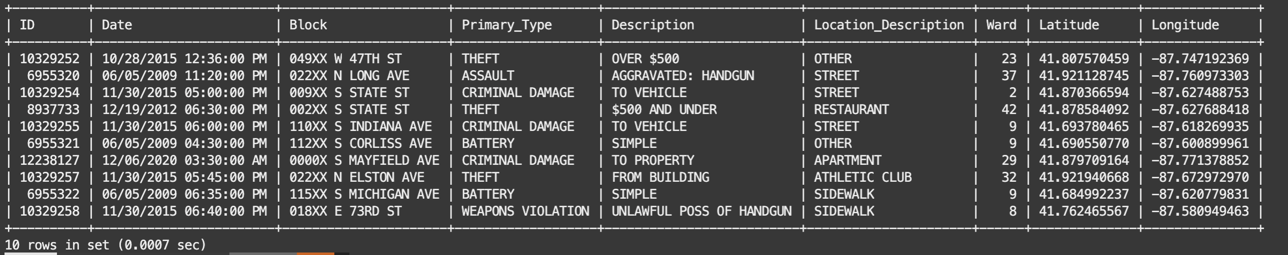
and then issue this query at the SQL prompt to view a few rows of relevant columns from the just-created crimes table:
select ID, Date, Block, Primary_Type, Description, Location_Description, Ward, Latitude, Longitude from crimes limit 10;
whose output is shown in Figure 1.
Prep Data for Machine Learning
The just-created crimes database table is transactional data that tracks the particulars of nearly 8 million individual crimes that occurred across Chicago during the past 20 years. To train a machine learning (ML) model that will forecast the frequency of those events, we first need to aggregate that transactional data across Chicago’s 50 geographic Wards (ie voting districts), which is performed using mysqlsh on the bastion VM to instruct MySQL Heatwave to execute the prep_data.sql script via
mysqlsh –user=admin –host=$host –sql < prep_data.sql
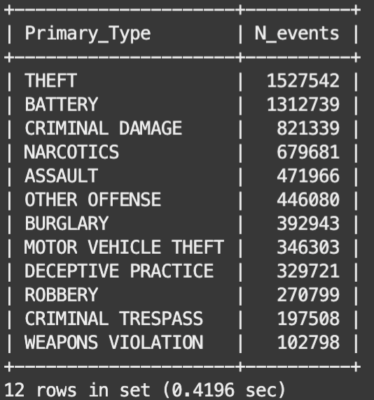
That script aggregrates 20 years of weekly crime-counts for Chicago’s twelve most frequent Primary_Types (crimes) that occurred across Chicago’s 50 Wards, with those results stored in the weekly_crimes table. To see the distribution of those top crimes, start an interactive mysqlsh session and then issue this query
select Primary_Type, sum(N_current) as N_events from weekly_crimes group by Primary_Type order by N_events desc;
whose output is shown in Figure 2.
The prep_data.sql script then splits the weekly_crimes table into a training sample (which is a random two-thirds sample of all records that were generated prior to year 2023), a testing sample (the remaining one-third of all pre-2023 records), as well as a validation sample containing all records generated during year 2023. Note that the validation sample of records are contiguous, which will allow us to generate timeseries plots that compare forecasted predictions to actual crime-counts.
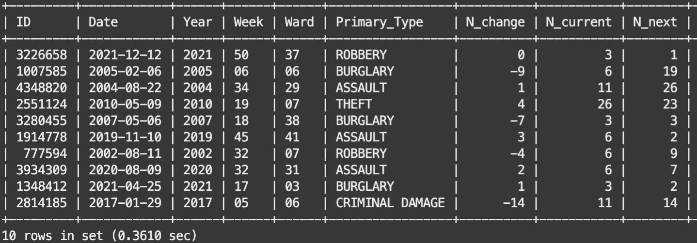
Figure 3 shows ten records from the training table of data that was generated by the prep_data.sql script. That table records the total number (N_current) of each Primary_Type (aka crime) that were committed across each of Chicago’s various Wards during various 7-day weeks that begin on the indicated Date. N_change is the week-to-week change of each Ward’s various crimes (ie N_change = N_current – last week’s N_current), and N_next is next week’s crime-count that is generated via MySQL’s lead() function operating on the N_current column, eg
lead(N_current, 1) over (partition by Ward, Primary_Type order by Date)
Which is the target variable for the regression algorithm that will be trained below, which will use the known Year, Week, Ward, Primary_Type, N_change, and N_current quantities to forecast next week’s crime-counts (N_next), for each Ward and Primary_Type.
AutoML for In-Database Machine Learning
Next, use the following code snippet to instruct AutoML to train a regression algorithm on the Chicago.train sample of records to predict column N_next, with AutoML explicitly instructed to ignore the ID and Date columns:
CALL sys.ML_TRAIN(
‘Chicago.train’,
‘N_next’,
JSON_OBJECT(
‘task’, ‘regression’,
‘exclude_column_list’, JSON_ARRAY(‘ID’, ‘Date’)
),
@next_model);
The arguments to the above call to sys.ML_TRAIN()provide AutoML with the name of the table containing the training data, the table column that is the model’s target variable, and tells AutoML that this is a regression task, and instructs AutoML to ignore the ID and Date columns, and then to store the unique name of the best-performing model in variable @next_model. Upon execution, AutoML then proceeds to launch numerous ML model-training experiments in parallel using the MySQL cluster’s available cpus, with AutoML using those experiments’ outcomes to select the best ML algorithm, to perform feature selection, and to optimize the ML algorithm’s various hyperparameters. Writing code to manually optimize all of the above often takes hours or days or more to develop/debug/test, while the above AutoML call executes those tasks in about 5 minutes and returns a very nicely optimized model.
To confirm the above, execute
SELECT QEXEC_TEXT FROM performance_schema.rpd_query_stats WHERE QUERY_TEXT=’ML_TRAIN’ ORDER BY QUERY_ID DESC limit 1;
which tells MySQL to report the various quantities that are associated with the just-trained model, but the principal fact that we need from that report is the model_handle, which for the author’s model is
“model_handle”: “Chicago.train_admin_1694470413”
which is the unique name of the AutoML-optimized model. Then use the following
set @next_model=’Chicago.train_admin_1694470413′;
select * from ML_SCHEMA_admin.MODEL_CATALOG where (model_handle=@next_model);
to select the desired record in MySQL Heatwave’s model-catalog, which tells us that the AutoML’s preferred algorithm is an LGBMRegressor, and that
“selected_column_names”: [“N_change”, “N_current”, “Primary_Type”, “Ward”, “Week”, “Year”],
which indicates that AutoML did not drop any features. The following,
CALL sys.ML_MODEL_LOAD(@next_model, NULL);
CALL sys.ML_SCORE(‘Chicago.test’, ‘N_next’, @next_model, ‘r2’, @score, NULL);
select @score;
then tells us that this model has an excellent R2=0.9 score, and that the model’s negative-mean-squared-errors,
CALL sys.ML_SCORE(‘Chicago.test’, ‘N_next’, @next_model, ‘neg_mean_squared_error’, @score, NULL);
select @score;
CALL sys.ML_SCORE(‘Chicago.train’, ‘N_next’, @next_model, ‘neg_mean_squared_error’, @score, NULL);
select @score;
are both very similar when computed on the test and train samples, which tells us that the AutoML-optimized model does not suffer from significant overfitting.
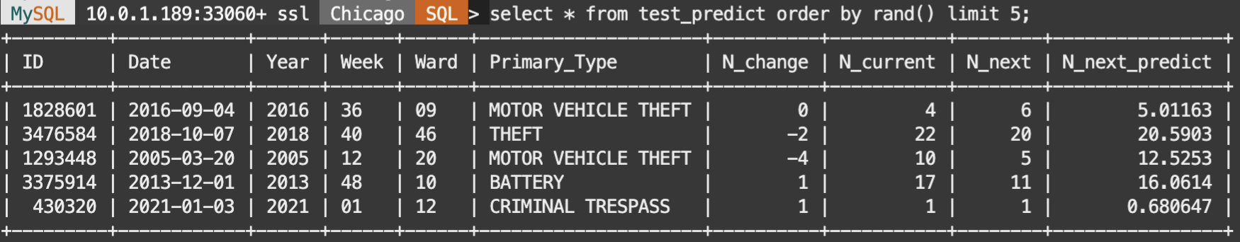
Then use the following,
drop table if exists test_predict_json;
CALL sys.ML_PREDICT_TABLE(‘Chicago.test’, @next_model, ‘Chicago.test_predict_json’, NULL);
drop table if exists test_predict;
create table test_predict as
select ID, Date, Year, Week, Ward, Primary_Type, N_change, N_current, N_next, Prediction as N_next_predict from test_predict_json;
select * from test_predict order by rand() limit 5;
to append a column of predictions to the test sample of records, with that result stored as table test_predict, of which five records are shown in Figure 4.
Then generate model predictions on the validation records via
drop table if exists valid_predict_json;
CALL sys.ML_PREDICT_TABLE(‘Chicago.valid’, @next_model,’Chicago.valid_predict_json’, NULL);
drop table if exists valid_predict;
create table valid_predict as
select ID, Date, Year, Week, Ward, Primary_Type, N_change, N_current, N_next, Prediction as N_next_predict from valid_predict_json;
The above code snippets illustrate how fast and easy it is to use AutoML to train and optimize an ML model on in-database data, to use that model to make predictions on the test and validation data samples, and to push those model predictions back into the database. The following subsection will then use python code executing on the bastion host to connect to the MySQL Heatwave cluster, query the test_predict table, and then generate a scatterplot that compares model predictions to actuals with much greater rigor. That step will also illustrate how other processes/services/applications that are external to the MySQL Heatwave cluster can interact with the in-database ML model, which effectively operationalizes that ML model by making its predictions visible to the broader business community via some simple code.
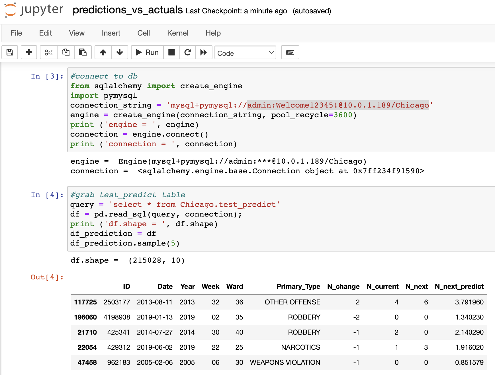
Use Jupyter on Bastion VM to Validate the ML model
Use the OCI console’s Cloud Shell to ssh into the bastion VM, and then install Anaconda python plus a few other python libraries including Jupyter, per these instructions. This installs all required python libraries within a python environment named ‘mysql’. Those same instructions also direct you to clone this experiment’s gitlab archive to the bastion VM, so navigate to that archive, activate the just-installed python environment, and then start the Jupyter server via
cd ~/mysql-heatwave-demo
conda activate mysql
jupyter notebook –certfile=~/jupyter-cert.pem –keyfile=~/jupyter-key.key
Then use your desktop’s browser to access the VM’s Jupyter server, which for this blog author is at https://132.145.171.157:8888, but keep in mind that you will have to tailor that URL to refer to your VM’s public IP. Then navigate to the predictions_vs_actuals.ipynb notebook and click Kernel > Restart & Run All to execute that Jupyter notebook. Figure 5 shows a key part of that notebook, which connects the Jupyter session that is running on the bastion VM to the MySQL Heatwave cluster, and to query the test_predict table that contains the model predictions that were generated earlier.
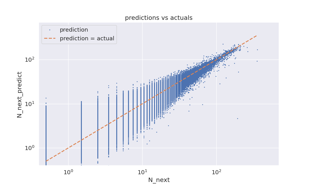
That notebook then provides a spot-check of the ML model’s accuracy by plotting a standard predictions-versus-actuals scatterplot, which is simply a plot of the model predictions column, N_next_predict, versus that model’s target column, N_next, Figure 6. Dashed line indicates where dots would lie if predictions equalled the actuals, and the fact that the predictions (blue dots) are uniformly scattered about the dashed line tells us that, on average, the model predictions do indeed track with Chicago’s actual crime-counts. That the scatter in the predictions also narrows when actual counts are larger tells us that predictions get more accurate when/where the signal in the target variable is larger. Which are all good indicators of AutoML having trained a reasonably accurate ML model.
The above illustrates how to interact with the ML model using MySQL commands communicated programmatically via the mysqlsh client, or using python code running inside of a Jupyter notebook that is external to the MySQL Heatwave cluster. All of which could be extended further to operationalize the MySQL Heatwave model across the rest of the business community via scripts or scheduled batch-jobs. However the majority of users will not want to write code to access those model predictions, and for those users the following section illustrates how to use a code-free tool like Oracle Analytics Cloud (OAC) to do such.
Oracle Analytics Cloud for Code-Free Access to ML model predictions
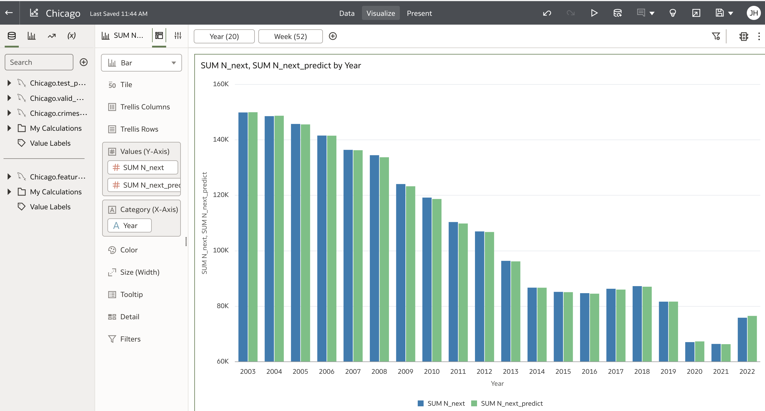
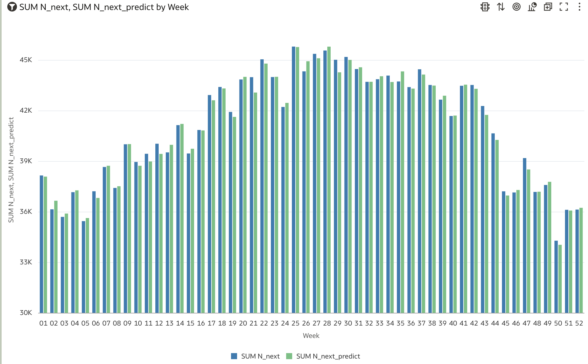
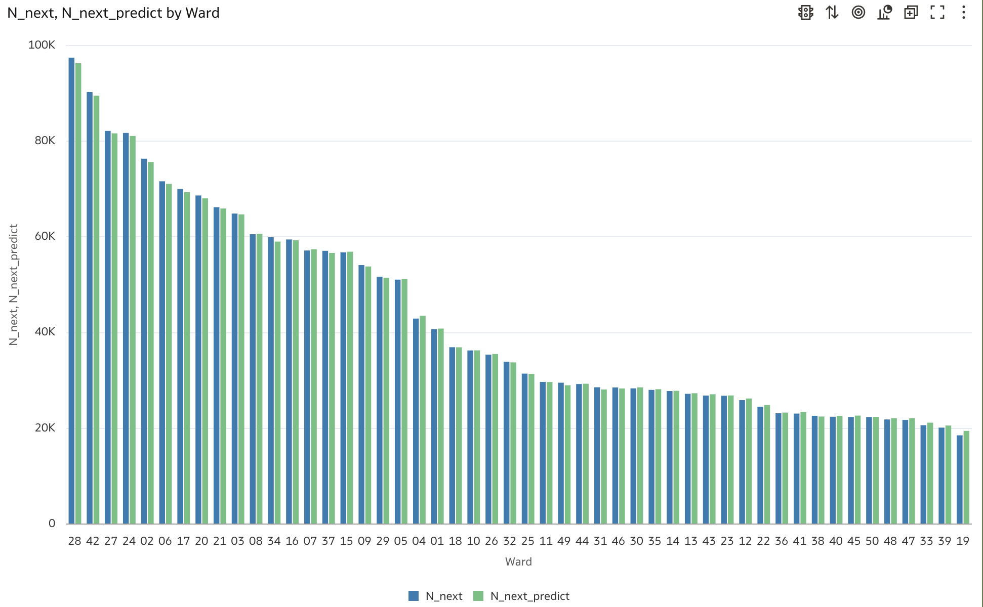
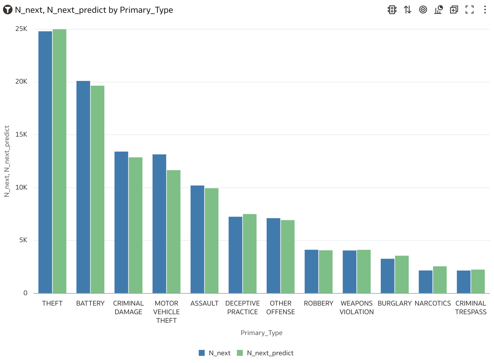
Next, launch a small Oracle Analytics Cloud (OAC) instance, connect it to the MySQL Heatwave cluster per these instructions, and then load the OAC workbook Chicago.dva into your OAC instance to generate several OAC charts that compare ML model predictions to actual crime-counts. To verify visually that the ML model’s weekly forecasts compare well to actuals, see Figure 7 for a comparison of yearly sums of Chicago’s crime-counts to annual sums of the predictions, with that plot showing that the ML model’s predictions do indeed recover Chicago’s year-over-year crime trends. Figure 8 compares weekly counts against predicted, which shows that the ML model reproduces Chicago’s seasonal crime trends, and Figure 9 shows that the model also exhibits the same variations in crime that the city sees across its various geographic Wards, with Figure 10 showing that model predictions vary as expected versus Primary_Type.
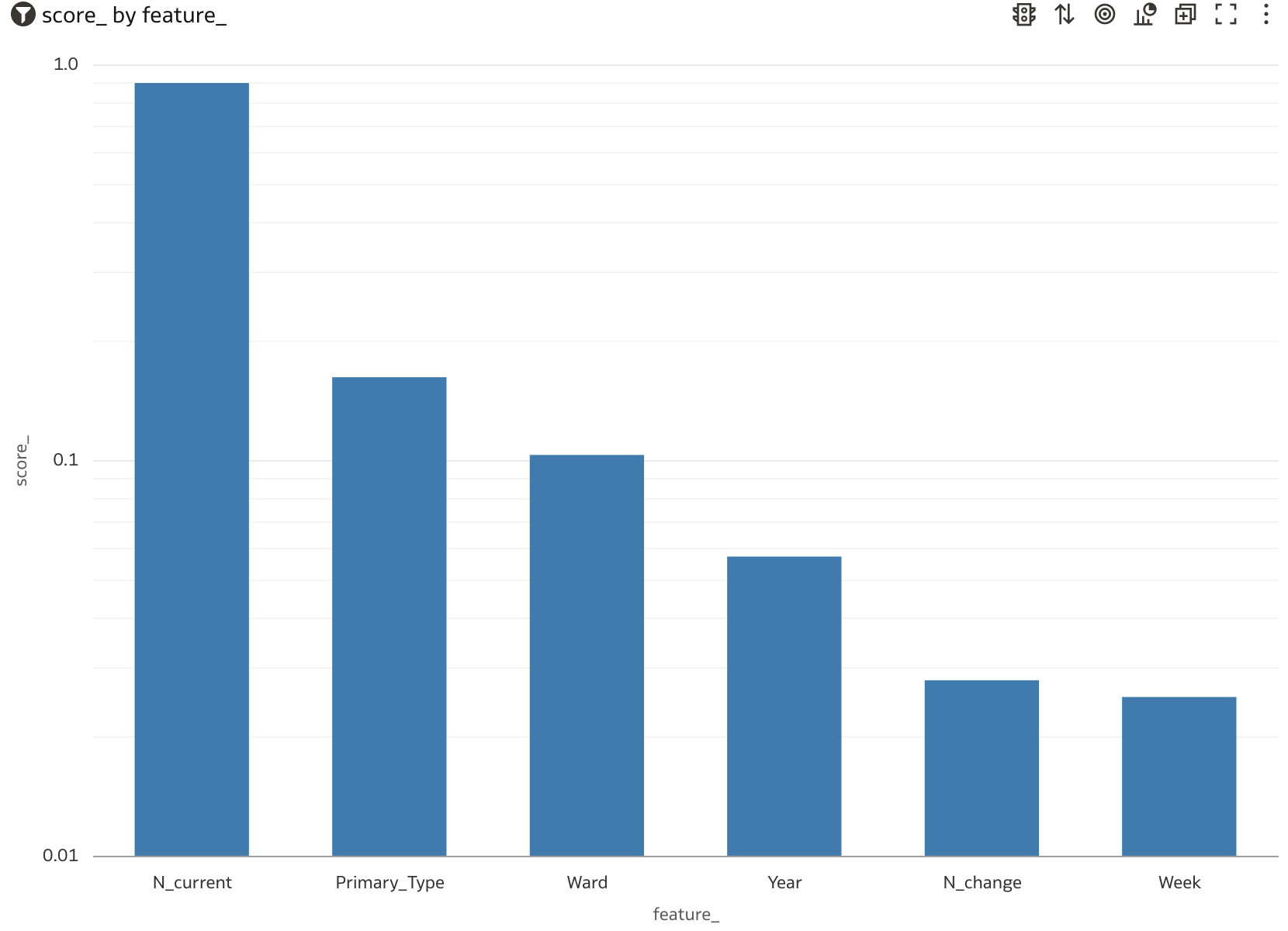
Model Feature Importance
OAC can also be used to visualize the ML model’s feature-importance. To see those feature-importance values at the mysqlsh command line, execute the following
CALL sys.ML_MODEL_LOAD(@next_model, NULL);
SELECT model_explanation FROM ML_SCHEMA_admin.MODEL_CATALOG WHERE (model_handle=@next_model);
and note that the output generated by the above, {“permutation_importance”: {“Ward”: 0.1035, “Week”: 0.0253, “Year”: 0.0573, “N_change”: 0.0279, “N_current”: 0.9013, “Primary_Type”: 0.1627}, is a json string. So use the following code snippet to parse that json
drop table if exists model_feature_importance;
create table model_feature_importance as
select ‘Ward’ as feature_, cast(json_extract(json, ‘$.Ward’) as float(8)) as score_ from
(select json_extract(model_explanation, ‘$.permutation_importance’) as json from
(SELECT model_explanation FROM ML_SCHEMA_admin.MODEL_CATALOG WHERE (model_handle=@next_model)) as T) as TT
union
select ‘Week’ as feature_, cast(json_extract(json, ‘$.Week’) as float(8)) as score_ from
(select json_extract(model_explanation, ‘$.permutation_importance’) as json from
(SELECT model_explanation FROM ML_SCHEMA_admin.MODEL_CATALOG WHERE (model_handle=@next_model)) as T) as TT
union
select ‘Year’ as feature_, cast(json_extract(json, ‘$.Year’) as float(8)) as score_ from
(select json_extract(model_explanation, ‘$.permutation_importance’) as json from
(SELECT model_explanation FROM ML_SCHEMA_admin.MODEL_CATALOG WHERE (model_handle=@next_model)) as T) as TT
union
select ‘Primary_Type’ as feature_, cast(json_extract(json, ‘$. Primary_Type’) as float(8)) as score_ from
(select json_extract(model_explanation, ‘$.permutation_importance’) as json from
(SELECT model_explanation FROM ML_SCHEMA_admin.MODEL_CATALOG WHERE (model_handle=@next_model)) as T) as TT
union
select ‘N_change’ as feature_, cast(json_extract(json, ‘$.N_change’) as float(8)) as score_ from
(select json_extract(model_explanation, ‘$.permutation_importance’) as json from
(SELECT model_explanation FROM ML_SCHEMA_admin.MODEL_CATALOG WHERE (model_handle=@next_model)) as T) as TT
union
select ‘N_current’ as feature_, cast(json_extract(json, ‘$.N_current’) as float(8)) as score_ from
(select json_extract(model_explanation, ‘$.permutation_importance’) as json from
(SELECT model_explanation FROM ML_SCHEMA_admin.MODEL_CATALOG WHERE (model_handle=@next_model)) as T) as TT
and to push the parsed feature importance scores into a new database table that is visible to OAC, Figure 11, to illustrate graphically which of the model’s various features are the most important drivers of outcomes.
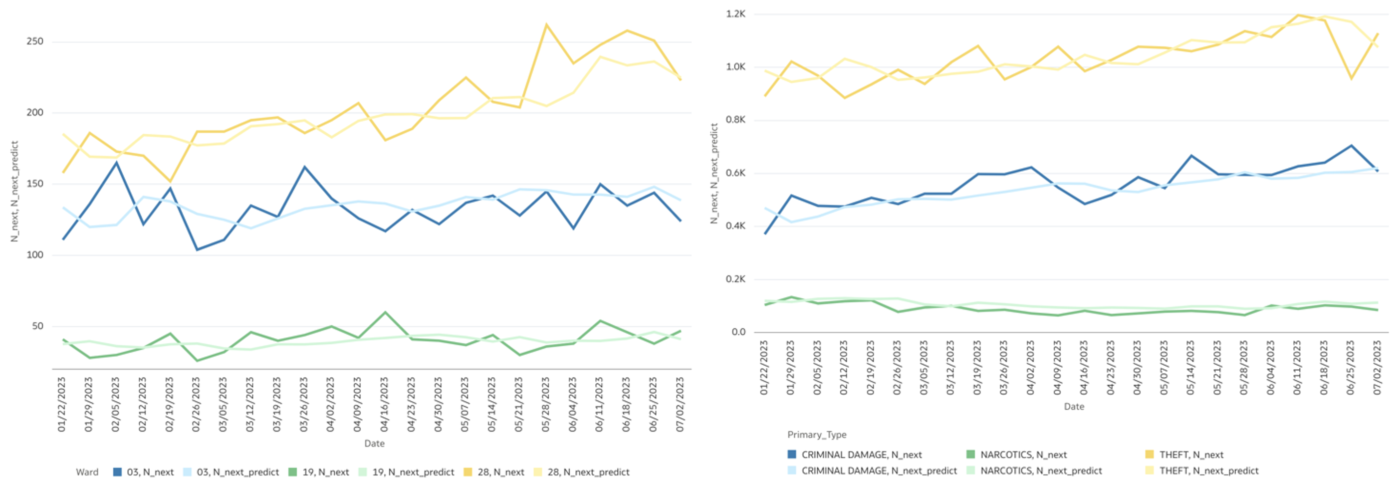
This experiment’s final model-validation chart is Figure 12, which shows timeseries plots of actual crime-counts over time alongside the ML model forecast that was generated on the 2023 validation dataset.
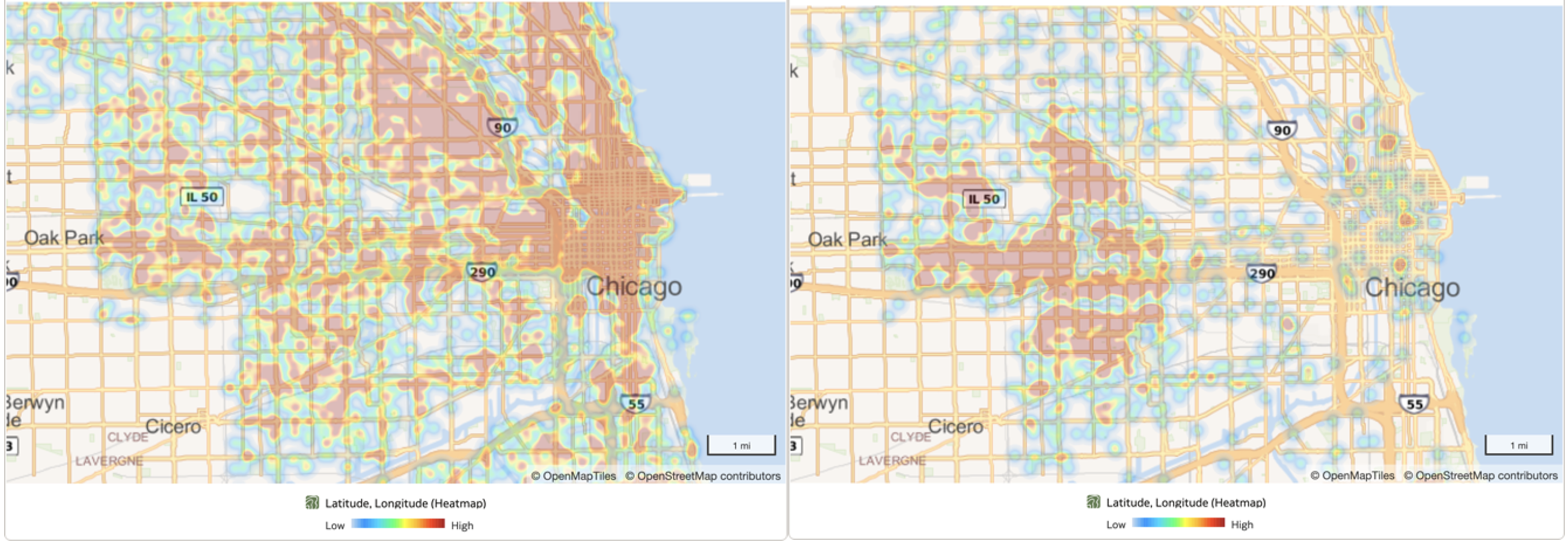
And because the Chicago dataset also provides geospatial Latitude and Longitude coordinates, it is straightforward to use OAC’s heatmap capability to show where various events occur across a Chicago streetmap, Figure 13.
Next Steps
If you have read this far, then you are presumably interested in MySQL Heatwave and in-database machine learning. So try it. Create an OCI tenancy and provision a small MySQL Heatwave cluster. Try using this blog post and its content, archived here, as a guide for loading data into that cluster, for using AutoML to train an ML model on that data, and then using Jupyter and/or OAC to visualize that model’s predictions and to assess their accuracies. A cloud-savvy individual could rebuild this exercise in a few hours, and that would result in an OCI bill of about $10 according to this OCI cost estimator. Once done, then think about whether MySQL Heatwave can help you and your business organization achieve their goals in in-database analytics. And if so, then please reach to Oracle, so that our experts can help yours to use MySQL-HW to attain those goals faster.
For additional information about the topics mentioned in this blog post, please see these resources:
- MySQL Heatwave
- Chicago crime data
- MySQL Heatwave Users Guide
- MySQL AutoML
- MySQL Heatwave Lakehouse
- code archive
- Anaconda python
- Jupyter
- mysqlsh
- Oracle Analytics Cloud
- OCI tenancy
Dataset disclaimer: This blog post and the codes referenced here use data that has been modified for use from its original source, www.cityofchicago.org, which is the official website of the City of Chicago. The City of Chicago makes no claims as to the content, accuracy, timeliness, or completeness of any of the data provided at this site. The data provided at this site is subject to change at any time. It is understood that the data provided at this site is being used at one’s own risk.