In the first post, we exported MySQL OpenTelemetry metrics directly to Prometheus. In the second, we used DBA questions to decide which metrics matter. This post turns those questions into a Grafana dashboard.

The objective is not to display every available metric. It is to make the next investigation obvious. When workload changes, a DBA should be able to decide whether the pressure is in connections, cache behavior, the write path, lock contention, or the host.

Build one dashboard around six operational questions

Use one dashboard, named MySQL Telemetry Overview in this example. The dashboard is organized around six operational questions. Each question is answered by one or more Grafana panels.

#	Operational question	Representative panels
1	Are connections rising or being refused?	Connections Connection rejections
2	Has workload changed?	Workload
3	Is the buffer pool serving reads efficiently?	Buffer Pool Hit Ratio Physical Reads
4	Is the write path under pressure?	Redo Write Throughput Redo Log Waits Pending Redo Fsyncs
5	Are transactions waiting for row locks?	Current Row Lock Waits Row Lock Wait Rate
6	Is the host contributing to the problem?	CPU Utilization Available Memory Average Disk Read and Write Time Network Traffic

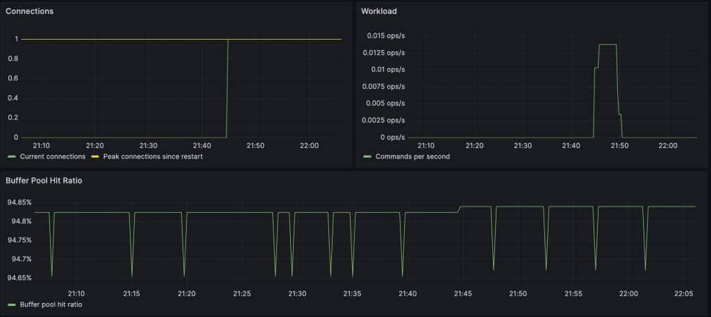
The dashboard can contain more than six panels. The six questions are the design model, while a panel is a Grafana implementation detail. The figures below show the related portions of one dashboard at a readable size.

Figure 1. Connections, workload, and buffer pool efficiency in the MySQL Telemetry dashboard. — *Figure 1. Correlating connections, workload, and buffer pool efficiency.*

Before building panels

Part 1 configured MySQL to export native telemetry through OTLP to the Prometheus OTLP receiver. Confirm that the meter groups required for the dashboard are enabled before creating Grafana panels.

SELECT NAME, ENABLED, FREQUENCY
FROM performance_schema.setup_meters
WHERE NAME IN (
  'mysql.stats',
  'mysql.stats.connection',
  'mysql.stats.com',
  'mysql.inno',
  'mysql.inno.buffer_pool'
);

In the test environment, MySQL exports these meters every 10 seconds. The exact Prometheus names depend on the OTLP receiver and any transformation performed between MySQL and Prometheus. Use Grafana Metrics browser or the Prometheus expression browser to confirm the metric names in the target environment before copying a query.

The examples below use the names observed when MySQL exports directly to the Prometheus OTLP receiver. For counter instruments, Prometheus appends _total.

For a dashboard that monitors more than one MySQL server, create an instance template variable and select one active instance for the panels below.

job="mysql/mysqld", instance="$instance"

This keeps each panel scoped to one MySQL server and avoids unintentionally combining time series from multiple instances.

Connections and workload

Start at the top of the dashboard with demand and connection activity.

Connections

Create a Time series panel named Connections.
Add the following queries.

threads_connected{
  job="mysql/mysqld",
  instance="$instance"
}

Set the legend to Current connections.

max_used_connections{
  job="mysql/mysqld",
  instance="$instance"
}

Set the legend to Peak connections since restart.
Set the unit to short.
max_used_connections is a post-restart high-water mark, not the configured max_connections limit. It is useful for capacity planning, but it does not by itself show headroom.

Connection rejections

Create a Stat panel named Connection rejections.

increase(
  errors_max_connections_total{
    job="mysql/mysqld",
    instance="$instance"
  }[5m]
)

Set Value to Last not null and Unit to short.

A value of zero is healthy. Any nonzero value means that MySQL has already refused client connections because the configured connection limit was reached.

Workload

Create a Time series panel named Workload.

rate(
  questions_total{
    job="mysql/mysqld",
    instance="$instance"
  }[5m]
)

Set the legend to Commands per second.
Set the unit to Throughput / ops/sec (ops).
questions_total is the MySQL command counter for statements sent by clients. The rate makes changes in client demand visible over time.

Traffic alone does not prove a problem. Read it with connection activity, application latency, and the following cache, write-path, and contention panels.

Buffer pool behavior

The Buffer Pool view needs two panels. The first establishes cache efficiency, and the second shows physical disk reads.

Buffer Pool Hit Ratio

Create a Time series panel named Buffer Pool Hit Ratio Since Restart.

1 - (
  reads_total{
    job="mysql/mysqld",
    instance="$instance"
  }
  /
  read_requests_total{
    job="mysql/mysqld",
    instance="$instance"
  }
)

Set the legend to Buffer pool hit ratio.
Set the unit to Percent (0.0-1.0).
The MySQL sources are Innodb_buffer_pool_reads and Innodb_buffer_pool_read_requests.

Part 2 used a rate-based expression to illustrate changes over a time window. For this lightly loaded test environment, this dashboard deliberately uses the cumulative ratio since restart because a short rate window can be dominated by only a few reads.

For a production workload, compare the baseline ratio with physical-read rate and application read latency before concluding that cache behavior caused a problem.

Physical Reads

Create a Time series panel named Physical Reads.

rate(
  reads_total{
    job="mysql/mysqld",
    instance="$instance"
  }[5m]
)

Set the legend to Physical reads per second.
Set the unit to Throughput / ops/sec (ops).

An increase in physical reads is more meaningful when it coincides with a fall from the usual hit-ratio baseline and higher read latency.

Write path and contention

The write path should be read as a group of signals. Redo throughput describes activity. Redo waits and pending fsyncs indicate whether that activity is creating sustained pressure.

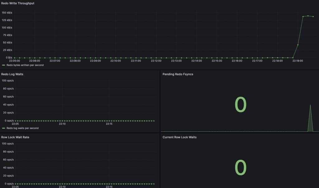
Redo Write Throughput

Create a Time series panel named Redo Write Throughput.

rate(
  os_log_written_total{
    job="mysql/mysqld",
    instance="$instance"
  }[5m]
)

Set the legend to Redo bytes written per second.
Set the unit to Data rate / bytes/sec (SI).

os_log_written is useful here because it turns redo activity into a time series.

Redo Log Waits

Create a Time series panel named Redo Log Waits.

rate(
  log_waits_total{
    job="mysql/mysqld",
    instance="$instance"
  }[5m]
)

Set the legend to Redo log waits per second.
Set the unit to Throughput / ops/sec (ops).

log_waits is sourced from Innodb_log_waits and records waits caused by a small log buffer.

Pending Redo Fsyncs

Create a Stat panel named Pending Redo Fsyncs.

os_log_pending_fsyncs{
  job="mysql/mysqld",
  instance="$instance"
}

Set Value to Last not null and Unit to short.

Keep the sparkline enabled. The large value is the current queue depth, while the sparkline shows whether an earlier burst drained quickly or persisted.

Lock contention

Create a Stat panel named Current Row Lock Waits.

row_lock_current_waits{
  job="mysql/mysqld",
  instance="$instance"
}

Set Value to Last not null and Unit to short.
Then create a Time series panel named Row Lock Wait Rate.

rate(
  row_lock_waits_total{
    job="mysql/mysqld",
    instance="$instance"
  }[5m]
)

Set the legend to Row lock waits per second.
Set the unit to Throughput / ops/sec (ops).

Use these panels to distinguish a transient wait from accumulating contention. If either signal rises with application latency, use Performance Schema to identify the sessions, statements, transactions, and objects involved.

Add system context with node_exporter

MySQL Telemetry describes the database server. Host CPU, memory, disk, and network signals require host telemetry. For this example, node_exporter runs on the MySQL host and Prometheus scrapes it with a separate node-mysql job.

- job_name: 'node-mysql'
  static_configs:
    - targets: ['MYSQL_PRIVATE_IP:9100']

This scrape job is complementary to MySQL’s direct OTLP export. It does not insert an OpenTelemetry Collector between MySQL and Prometheus.

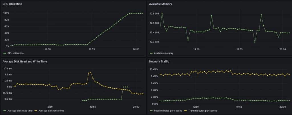
Figure 3. Host-level system context for the MySQL server. — *Figure 3. CPU, available memory, disk activity, and network traffic provide the host-level context needed to interpret MySQL telemetry.*

CPU Utilization

Create a Time series panel named CPU Utilization.

100 * (
  1 - avg by (instance) (
    rate(node_cpu_seconds_total{
      job="node-mysql",
      mode="idle"
    }[5m])
  )
)

Set the legend to CPU utilization.
Set the unit to Percent (0-100).

Available Memory

Create a Time series panel named Available Memory.

node_memory_MemAvailable_bytes{job="node-mysql"}

Set the legend to Available memory.
Set the unit to Data / bytes (IEC).

MemAvailable includes memory Linux can make available without swapping, including reclaimable page cache. It is more useful for this purpose than raw free memory.

Average Disk Read and Write Time

Create a Time series panel named Average Disk Read and Write Time with these two queries.

Query A — read time

1000 * (
  sum by (instance) (
    rate(node_disk_read_time_seconds_total{
      job="node-mysql",
      device!~"loop.*|ram.*|fd.*|sr.*"
    }[5m])
  )
  /
  sum by (instance) (
    rate(node_disk_reads_completed_total{
      job="node-mysql",
      device!~"loop.*|ram.*|fd.*|sr.*"
    }[5m])
  )
)

Set the legend to Average disk read time.

Query B — write time

1000 * (
  sum by (instance) (
    rate(node_disk_write_time_seconds_total{
      job="node-mysql",
      device!~"loop.*|ram.*|fd.*|sr.*"
    }[5m])
  )
  /
  sum by (instance) (
    rate(node_disk_writes_completed_total{
      job="node-mysql",
      device!~"loop.*|ram.*|fd.*|sr.*"
    }[5m])
  )
)

Set the legend to Average disk write time.
Set the unit to Time / milliseconds (ms).

The Linux disk counters record the cumulative time spent in read and write operations separately. Dividing each time rate by its completed-operation rate produces an I/O-weighted average time per completed read or write across the selected devices.

These are host-level service-time signals, not end-to-end storage-latency measurements. Use them as context alongside MySQL redo, lock, and application-latency signals; queueing and concurrent I/O can change the interpretation.

Network Traffic

Create a Time series panel named Network Traffic.
Add a receive query.

sum(
  rate(node_network_receive_bytes_total{
    job="node-mysql",
    device!~"lo|docker.*|veth.*|br-.*"
  }[5m])
)

Set the legend to Receive bytes per second.
Add a transmit query.

sum(
  rate(node_network_transmit_bytes_total{
    job="node-mysql",
    device!~"lo|docker.*|veth.*|br-.*"
  }[5m])
)

Set the legend to Transmit bytes per second.
Set the unit for the panel to Data rate / bytes/sec (SI).

Read the dashboard in sequence

When an application slows down, start with the question that changes the next decision.

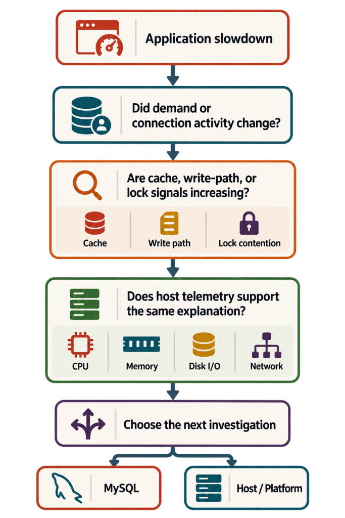
The dashboard guides the next investigation. It does not replace root-cause analysis. In the next post, we will use the same signals to move from dashboard symptoms to concrete MySQL troubleshooting evidence.

Visualizing MySQL Telemetry with Grafana

Build one dashboard around six operational questions

Before building panels

Connections and workload

Connections

Connection rejections

Workload

Buffer pool behavior

Buffer Pool Hit Ratio

Physical Reads

Write path and contention

Redo Write Throughput

Redo Log Waits

Pending Redo Fsyncs

Lock contention

Add system context with node_exporter

CPU Utilization

Available Memory

Average Disk Read and Write Time

Network Traffic

Read the dashboard in sequence

References

Machiko Ikoma

MySQL Principal Solution Engineer

Making Sense of MySQL Telemetry Metrics

Visualizing MySQL Telemetry with Grafana

Build one dashboard around six operational questions

Before building panels

Connections and workload

Connections

Connection rejections

Workload

Buffer pool behavior

Buffer Pool Hit Ratio

Physical Reads

Write path and contention

Redo Write Throughput

Redo Log Waits

Pending Redo Fsyncs

Lock contention

Add system context with node_exporter

CPU Utilization

Available Memory

Average Disk Read and Write Time

Network Traffic

Read the dashboard in sequence

References

Authors

Machiko Ikoma

MySQL Principal Solution Engineer

Making Sense of MySQL Telemetry Metrics