With the release of MySQL 9.7 Community Edition, the Hypergraph Optimizer is now available to everyone. This is a significant addition to MySQL and one that has generated a lot of excitement in the MySQL community. The promise is simple: better execution plans for complex queries, especially those with many joins.

Like most new features, though, it comes with an important question: should you just turn it on and forget about it?

The short answer is no.

In this post, we’ll look at what a query optimizer actually does, how the traditional MySQL optimizer differs from the Hypergraph Optimizer, and, most importantly, examine a real-world example where the Hypergraph Optimizer improves performance and discuss why it isn’t necessarily the best optimizer for every workload. By the end, you should have a good understanding of when Hypergraph is likely to help and when it’s better to let MySQL’s traditional optimizer choose the execution plan.

What is a Query Optimizer?

Every time you submit a SQL statement, the database has to decide how it is going to execute it. While there is only one correct answer to your query, there are often dozens, hundreds, or even thousands of different ways to get there.

That’s where the query optimizer comes in.

Its job is to find the most efficient execution plan by considering things like available indexes, table statistics, join order, and estimated row counts. The goal is simple: return the correct results while doing the least amount of work possible.

For simple queries, there usually aren’t many decisions to make. But once a query starts joining several tables together, the optimizer becomes incredibly important. Two execution plans can return exactly the same result, yet one may finish in milliseconds while another takes several seconds or even minutes. That’s why the optimizer is often considered one of the most critical pieces of any relational database.

Traditional Query Optimization vs. Hypergraph Optimization

One of the biggest jobs a query optimizer has is deciding the order in which tables should be joined. That might sound straightforward, but it quickly becomes complicated.

With two tables there are only a couple of possibilities. Add a few more tables and the number of possible join orders starts growing rapidly. By the time you’re joining ten or more tables, there are simply too many combinations to evaluate in a reasonable amount of time. Spending ten seconds finding the perfect execution plan isn’t very helpful if the query itself only runs for one second.

To solve this problem, MySQL’s traditional optimizer uses a cost-based approach along with a variety of heuristics to narrow the search space. Instead of evaluating every possible join order, it focuses on the ones most likely to produce a good execution plan. Most of the time, this works remarkably well.

The Hypergraph Optimizer takes a different approach. Rather than using the traditional join enumeration strategy, it models the query as a graph of relationships between tables. This allows it to explore a much larger set of possible join orders while still avoiding obviously poor choices. The result is that it can sometimes discover execution plans that the traditional optimizer would never consider.

Of course, there is no such thing as a free lunch.

Exploring more possible plans takes more optimization effort. For large analytical queries, that extra work can pay off with significantly faster execution. For smaller or simpler queries, there may not be enough join-order complexity for the Hypergraph Optimizer to discover a meaningfully better execution plan. In those cases, execution time may be nearly identical to the traditional optimizer, and occasionally the additional optimization effort can outweigh any benefit. In those cases, the traditional optimizer may perform just as well, or even better.

Enabling the Hypergraph Optimizer

One of the nice things about the Hypergraph Optimizer is that you don’t have to enable it globally just to see what it can do. MySQL provides several ways to enable Hypergraph, allowing you to test it at the level that makes the most sense for your environment.

The easiest approach is to enable Hypergraph for a single query using an inline optimizer hint:

SELECT /*+ SET_VAR(optimizer_switch='hypergraph_optimizer=on') */
…

This is my preferred approach when evaluating queries because it limits the change to a single statement. It also makes it easy to compare execution plans side by side, since the only difference between the two queries is the optimizer being used.

If you want to test a larger workload, Hypergraph can also be enabled for the current session:

SET SESSION optimizer_switch='hypergraph_optimizer=on';

Or, if you’ve completed your testing and want every new client connection to use Hypergraph by default, you can enable it globally:

SET GLOBAL optimizer_switch='hypergraph_optimizer=on';

For the examples in this article, I’ll use the inline optimizer hint. It keeps the comparison fair by ensuring the SQL, schema, and data remain exactly the same. The only thing that changes is the optimizer, making it much easier to see the impact of Hypergraph on the resulting execution plan.

Example Query

Now that we’ve covered the basics, let’s look at a query where the Hypergraph Optimizer has an opportunity to shine.

This example uses a reporting-style schema centered around sales_order and sales_line, with supporting tables for customers, products, sellers, and archived 2025 order data. While it isn’t a classic star schema, it represents the kind of transactional workload commonly found in e-commerce and order management systems. More importantly, the relationships between these tables give the optimizer multiple possible join paths, making join order a key factor in overall performance.

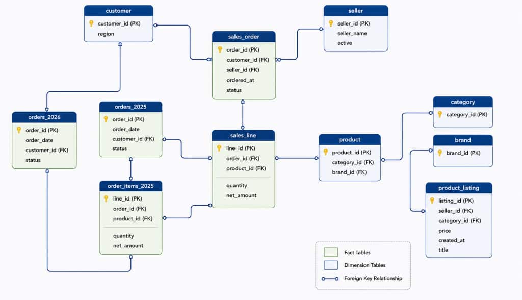
The query below summarizes current sales activity while comparing it against archived order data from 2025. It combines current and historical orders, joins across multiple lookup tables, and applies several selective predicates, including date ranges, order status, customer region, seller status, and product category.

Because there are multiple valid ways to join these tables, this is exactly the type of query where the Hypergraph Optimizer can explore alternative execution plans that the traditional optimizer may not consider.

SELECT COUNT(*) AS matched_lines,
   ROUND(SUM(sl.net_amount), 2) AS current_revenue
FROM sales_order so
JOIN sales_line sl ON sl.order_id = so.order_id
JOIN product p ON p.product_id = sl.product_id
JOIN customer c ON c.customer_id = so.customer_id
JOIN seller s ON s.seller_id = so.seller_id
JOIN orders_2025 o25 ON o25.customer_id = c.customer_id
JOIN order_items_2025 i25 ON i25.order_id = o25.order_id
JOIN product p25 ON p25.product_id = i25.product_id
               AND p25.category_id = p.category_id
WHERE so.ordered_at BETWEEN '2026-11-20' AND '2026-11-30'
  AND so.status = 'PAID'
  AND o25.order_date BETWEEN '2025-01-01' AND '2025-12-31'
  AND o25.status = 'PAID'
  AND c.region IN ('US','DE','NO')
  AND s.active = TRUE
  AND p.category_id IN (7,12,19,34)

Comparing the Execution Plans

Now for the interesting part. We ran the exact same query twice, once with MySQL’s traditional optimizer and once with the Hypergraph Optimizer enabled through the inline hint. The goal is to see whether Hypergraph can find a better path through the same data. The full JSON output can be viewed from the file below. The plans shown here were generated using EXPLAIN ANALYZE FORMAT=JSON, which reports actual execution statistics in addition to the optimizer’s chosen plan.

Traditional Optimizer

To see what the traditional optimizer is doing, we run the query with EXPLAIN ANALYZE FORMAT=JSON in front of it.

EXPLAIN ANALYZE FORMAT=JSON
SELECT COUNT(*) AS matched_lines,…

I like using JSON here because my brain finds it a little easier to follow than the classic output. It is still the same plan, just with fewer squinting opportunities.

Here is a visual representation of thsi execution plan.

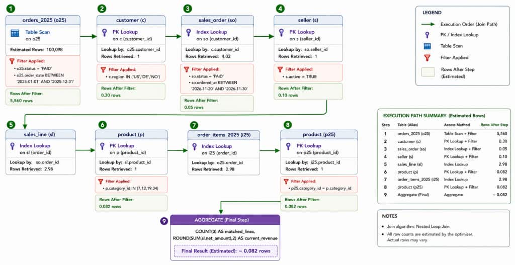
The traditional plan stays very close to the classic nested-loop style. It starts with a table scan on o25, filters that branch down to paid orders in the 2025 date range, and then joins to customer using a single-row primary key lookup. From there, it continues through sales_order, seller, sales_line, product, order_items_2025, and finally p25.

The most important details in the plan are:

• Table scan on `o25`
• Filter on `o25.status = ‘PAID’` and `o25.order_date`
• Single-row lookup on `customer`
• Index lookup on `sales_order` using `ix_customer`
• Single-row lookup on `seller`
• Index lookup on `sales_line` using `ix_order`
• Single-row lookup on `product`
• Index lookup on `order_items_2025` using `ix_order_id`
• Single-row lookup on `p25` using `PRIMARY`
• Final filter on `p25.category_id = p.category_id`

This plan does the job, but it keeps everything in a fairly linear nested-loop chain. The query finishes in about 451 ms.

Hypergraph Optimizer

Now let’s run the exact same query again, but this time we’ll enable the Hypergraph Optimizer using the inline optimizer hint we discussed earlier.

EXPLAIN ANALYZE FORMAT=JSON
SELECT /*+ SET_VAR(optimizer_switch='hypergraph_optimizer=on') */
COUNT(*) AS matched_lines, ...

Notice that the query itself hasn’t changed. The only difference is the inline hint, which tells MySQL to use the Hypergraph Optimizer just for this statement. This allows us to compare optimizer behavior directly, since the only variable is the optimizer itself.

Let’s look at the visual representation for the execution plan from Hypergraph.

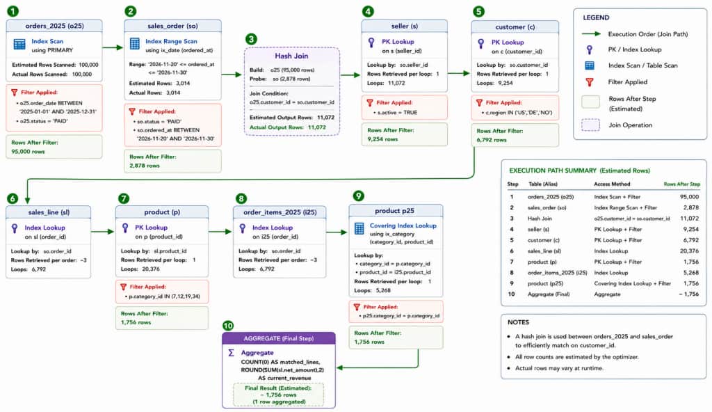
The Hypergraph plan takes a different route early on. Rather than simply following a linear nested-loop chain, it builds a hash table from one side of the join and uses an inner hash join on so.customer_id = o25.customer_id to combine the current and archived order branches. Reducing the number of rows flowing into subsequent joins helps explain why this execution plan completes significantly faster.

The useful parts of this plan are:

• Index scan on `o25` using `PRIMARY`
• Index range scan on `so` using `ix_date`
• Inner hash join on `so.customer_id = o25.customer_id`
• Single-row lookup on `seller`
• Single-row lookup on `customer`
• Index lookup on `sales_line` using `ix_order`
• Single-row lookup on `product`
• Index lookup on `order_items_2025` using `ix_order_id`
• Single-row covering lookup on `p25` using `ix_category`

This is the key difference worth showing in the blog. Hypergraph is not just doing the same thing with a different label. It changes the early join shape, and that version finishes in about 122 ms. More importantly, the improvement was achieved without making any changes to the SQL itself. The only difference between the two executions was the optimizer that chose the execution plan.

This example demonstrates the type of workload the Hypergraph Optimizer was designed to improve. Both optimizers produced a valid execution plan, but Hypergraph selected a different join strategy by introducing an early hash join and reordering portions of the join graph. That change reduced the overall execution time from approximately 451 ms to 122 ms, a performance improvement of nearly 4x.

While the original query wasn’t exactly slow, it was processing a relatively modest amount of data. As transactional systems grow and tables accumulate millions or even billions of rows, the efficiency of the execution plan becomes increasingly important. A query that completes in a fraction of a second today can become a bottleneck tomorrow if the optimizer is doing more work than necessary. By finding a more efficient join strategy, the Hypergraph Optimizer provides a plan that is better positioned to scale as the underlying data continues to grow.

The key takeaway from this example is that the Hypergraph Optimizer can discover execution strategies that significantly reduce query execution time for complex join workloads. When multiple join paths and selective predicates are present, giving the optimizer additional freedom to explore alternative plans can produce substantial performance gains.

Wrap-Up

The Hypergraph Optimizer is an important evolution of MySQL’s query optimizer. By exploring a broader set of possible join orders than the traditional optimizer, it can discover execution plans that substantially reduce the amount of work required for complex multi-table queries. As this example demonstrated, those improvements can translate into significantly lower execution times without requiring any changes to the SQL itself.

That said, it’s important to avoid thinking of the Hypergraph Optimizer as a universal performance switch. Like any cost-based optimizer, it makes decisions based on available statistics, estimated cardinalities, and the shape of the query. Some workloads will see dramatic improvements, others will see little or no difference, and in certain cases a query may even perform worse than it did with the traditional optimizer.

For that reason, enabling the Hypergraph Optimizer should be treated as an opportunity to measure and not an assumption that every query will become faster. Evaluate your most important queries using realistic data volumes and production-like workloads. A query that performs well against thousands of rows may behave very differently when executed against millions.

When comparing execution plans, use EXPLAIN ANALYZE whenever possible rather than relying solely on estimated costs. Estimated execution plans describe what the optimizer expects to happen, while EXPLAIN ANALYZE shows what actually happened during execution. Those real execution statistics provide a much more accurate picture of whether the optimizer’s decisions are paying off.

The Hypergraph Optimizer is another powerful tool in MySQL’s performance arsenal, providing MySQL with an additional strategy for solving complex join problems. Whether it becomes the best strategy for your workload depends not on theory, but on measurement. Test with representative data, validate with EXPLAIN ANALYZE, and let the results, and not assumptions, determine which optimizer delivers the best performance.