Did you know you can expose and analyze your data like a graph?
Graphs put relationships between entities in the focus of interest. They are ideally suited to model and analyze complex, deeply hierarchical, or circular relationships.
How can you do that?
Very simple. You first create a graph view of your data and then run pattern-matching queries to analyze your graph. Both steps use PGQL, a SQL-like syntax that is intuitive and, therefore, easy to use.
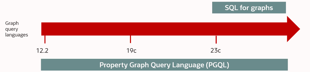
This post wants to give you a head start on using PGQL and Oracle Graph technologies with existing data residing in an Oracle Database 19c (or 12.2). Here is what you need:
- Ingredients:
- Data (stored in your Oracle Database)
- Tools:
- SQL Developer (link to download the current version) or
- SQLcl plus the PGQL plug-in (link to version 24.2)
Please note that with Oracle Database 23ai, working with graphs becomes even more straightforward. Why? Oracle has implemented SQL/PGQ, a new extension to the SQL:2023 standard supporting Property Graph Queries. You will see that the PGQL syntax is very similar to SQL/PGQ due to Oracle´s contribution to the standard definition. Therefore, the effort now to familiarize yourself with PGQL is not a waste of time.
(Note: The image still refers to 23c from when the article was published first. It is 23ai now.)
Now, are you ready to learn something you didn´t know before? Then, let´s get started.
Here is what we do:
- Download and install SQLcl and the PGQL plug-in.
- Load sample data into your Oracle Database using SQLcl.
- Create a graph model (view) of your data.
- Analyze your graph using SQLcl.
Step 1: Download and install SQLcl and the PGQL plugin
Use this link to download the latest version of SQLcl. Extract the zip file into a folder of your choice. The SQLcl utility resides in the ./sqlcl/bin folder.
You can now download the PGQL plug-in from Oracle Software Delivery Cloud (search for “Oracle Graph Server and Client”) or from Oracle Graph Server and Client Downloads.
To install the plug-in, you need to unzip the downloaded file into the lib/ext directory of your local SQLcl installation.
That´s it. Start SQLcl.
sql /nolog
Connect with a privileged user to create a new schema where you later store the sample data.
--------------------------------------------------------
-- Log into your Oracle Database instance using SYSTEM.
-- Adapt the following statements to your needs.
-- The new user is required to have the GRAPH_DEVELOPER role.
--------------------------------------------------------

connect system/Welcome2PGQL_1234#@localhost:1521/pdb1
create user graphuser identified by Welcome2PGQL_9876#;
grant graph_developer, create session, create table, create view to graphuser;
alter user graphuser quota unlimited on users;
Note: The GRAPH_DEVELOPER role is a convenient grouping of common roles like CONNECT and RESOURCE plus several roles with the prefix PGX_ that are required to work with Oracle Graph Server (commonly known as PGX Server).
Verify that you can connect with the newly created user.
connect graphuser/Welcome2PGQL_9876#@localhost:1521/pdb1
Step 2: Load sample data
Download the sample data from this folder available on GitHub. It contains two .csv files, named BANK_ACCOUNTS.csv and BANK_TXNS.csv.
Use your newly created database user to set up the tables.
--------------------------------------------------------
--  Create table BANK_ACCOUNTS
--------------------------------------------------------
create table bank_accounts (
    acct_id number(10),
    name varchar2(100),
      balance number(13,2)
)
/
--------------------------------------------------------
--  Add unique index to table BANK_ACCOUNTS
--------------------------------------------------------
create unique index bank_accounts_pk on bank_accounts (acct_id)
/
--------------------------------------------------------
--  Add primary key constraint to table BANK_ACCOUNTS
--------------------------------------------------------
alter table bank_accounts add constraint bank_accounts_pk primary key (acct_id)
/
--------------------------------------------------------
--  Create staging table BANK_TXNS_TEMP
--    to avoid problems with autogenerated transaction ID
--    during the data import
--------------------------------------------------------
create table bank_txns_temp (
      from_acct_id number(10),
      to_acct_id number(10),
      txn_date timestamp,
      amount number(13,2),
      currency varchar2(3)
)
/
--------------------------------------------------------
--  Create table BANK_TXNS
--------------------------------------------------------
create table bank_txns (
      txn_id number(10) generated always as identity,
      from_acct_id number(10),
      to_acct_id number(10),
      txn_date timestamp,
      amount number(13,2),
      currency varchar2(3)
)
/
--------------------------------------------------------
--  Add unique index to table BANK_TXNS
--------------------------------------------------------
create unique index bank_txns_pk on bank_txns (txn_id)
/
--------------------------------------------------------
--  Add primary key constraints to table BANK_TXNS
--------------------------------------------------------
alter table bank_txns add constraint bank_txns_pk primary key (txn_id)
/
--------------------------------------------------------
--  Add foreign key constraints to table BANK_TXNS
--------------------------------------------------------
alter table bank_txns add constraint bank_txns_from_acct_fk foreign key (from_acct_id) references bank_accounts(acct_id)
/
alter table bank_txns add constraint bank_txns_to_acct_fk foreign key (to_acct_id) references bank_accounts(acct_id)
/
Now, you can fill the tables with the downloaded sample data using SQLcl.
----------------------------------------------------------------------
-- Import data using LOAD
--    Load bank accounts directly
--    Load bank transactions into a staging table first
--    (to avoid errors related to the autogenerated transaction ID´s)
-- Adapt the

    to match the folder where the files are located

  ----------------------------------------------------------------------


set loadformat csv
-- Make sure to have the decimals in the data correctly interpreted
set load locale American America

-- Import data using LOAD
load table bank_accounts BANK_ACCOUNTS.csv
load table bank_txns_temp BANK_TXNS.csv

/* Expected results:

Load data into table GRAPHUSER.BANK_ACCOUNTS
#INFO Number of rows processed: 10.000
#INFO Number of rows in error: 0
#INFO Last row processed in final committed batch: 10.000
SUCCESS: Processed without errors

Load data into table GRAPHUSER.BANK_TXNS_TEMP
#INFO Number of rows processed: 50.000
#INFO Number of rows in error: 0
#INFO Last row processed in final committed batch: 50.000
SUCCESS: Processed without errors

*/

-- Verify transaction data in the staging table
select * from bank_txns_temp fetch first 10 rows only;

-- Copy data from staging table BANK_TXNS_TEMP into BANK_TXNS
insert into bank_txns (from_acct_id, to_acct_id, txn_date, amount, currency)(
    select from_acct_id, to_acct_id, txn_date, amount, currency from bank_txns_temp);
commit;

-- Verify that your data was loaded correctly
select * from bank_accounts fetch first 10 rows only;
select * from bank_txns fetch first 10 rows only;

-- Drop staging table BANK_TXNS_TEMP
drop table bank_txns_temp purge;
All statements should run without any errors. If this is not the case, check what´s wrong. The GitHub repository contains a script to clean up all created objects. Use it to start from scratch if needed.
Step 3: Create a graph model
PGQL provides a data definition language (DDL) to create graphs. To make sure that SQLcl from now on speaks PGQL instead of SQL, activate the plug-in:
pgql auto on;A graph consists of vertices (also called nodes) and edges. Both vertices and edges typically have labels and properties assigned. Properties are expressed as key-value-pairs.
The DDL statement to create a graph view on your existing two tables can look like the following:
CREATE PROPERTY GRAPH bank_graph
  VERTEX TABLES (
    bank_accounts
      KEY (acct_id)
      LABEL account
      PROPERTIES ( acct_id, name, balance )
  )
  EDGE TABLES (
    bank_txns
      KEY (txn_id)
      SOURCE KEY ( from_acct_id ) REFERENCES bank_accounts
      DESTINATION KEY ( to_acct_id ) REFERENCES bank_accounts
      LABEL transfers
      PROPERTIES ( txn_id, from_acct_id, to_acct_id, amount, txn_date )
  )
  OPTIONS (PG_PGQL);
The statement specifies
- the name of the graph,
- which tables serve as vertices,
- which tables serve as edges,
- which columns of the BANK_ACCOUNTS and BANK_TXNS tables are used as properties for further analysis,
- which labels are assigned to the vertices and edges,
- and the source format for the graph (PG_PGQL). Please note, that in previous PGQL versions the format was named PG_VIEW. It was changed to better distinguish with the new SQL-based Property Graph support in Oracle Database 23. The format for those graphs in named PG_SQL.
All details about the graph creation are stored in five metadata tables, starting with the name of the graph. For the newly created graph, those are:
- BANK_GRAPH_ELEM_TABLE$
- BANK_GRAPH_KEY$
- BANK_GRAPH_LABEL$
- BANK_GRAPH_PROPERTY$
- BANK_GRAPH_SRC_DST_KEY$
Make sure you do not alter the table contents. If you did, you will compromise further analysis of the graph. You find a detailed description of the CREATE PROPERTY GRAPH syntax in the documentation.
You are done with all preparation steps, which you need to do only once. You can now go ahead and analyze your graph.
Step 4: Query your data using the Property Graph Query Language
Let me start with a few words about PGQL:
Alongside familiar SQL constructs like SELECT, FROM, WHERE, GROUP BY, and ORDER BY, PGQL allows for matching fixed-length graph patterns and variable-length graph patterns. Fixed-length graph patterns match a fixed number of vertices and edges per solution. The types of the vertices and edges can be defined through arbitrary label expressions such as account|company, for example to match edges that have either the label account or the label company. This means that edge patterns are higher-level joins that can relate different types of entities at once. Variable-length graph patterns, on the other hand, contain one or more quantifiers like *,+,? or {2,4} for matching vertices and edges in a recursive fashion. This allows for encoding graph reachability (transitive closure) queries as well as shortest and cheapest path finding queries.
PGQL deeply integrates graph pattern matching with subquery capabilities so that vertices and edges that are matched in one query can be passed into another query for continued joining or pattern matching. Since PGQL is built on top of SQL’s foundation, it benefits from all existing SQL features and any new SQL features that will be added to the standard over time.
Coming back to our graph example, since the metadata structure that keeps the information about all created graphs is a graph of its own, we start with querying that metadata graph.
SELECT g.graph_name
FROM MATCH (g IS property_graph) ON property_graph_metadata
ORDER BY g.graph_name;
The result of this query is one row returning the name of the graph you created.
Let me explain the query syntax in more details based on the next simple, fixed-length path pattern matching query:
--------------------------------------------------------
-- Fixed-length path query example:
--   List 10 transactions between two accounts
--   that are directly connected via a transaction.
--------------------------------------------------------
SELECT
  a.acct_id as src_account,
  b.acct_id as dst_account,
  t.amount as txn_amount,
  t.txn_date as txn_date
FROM MATCH (a IS account)-[t IS transfers]->(b IS account) ON bank_graph
ORDER BY src_account, dst_account, txn_date
LIMIT 10;
In the query above
bank_graphis the name of the graph.(a IS account)and(b IS account)are vertex patterns in whichaandbare variable names andIS accounta label expression.[e IS transfers]is an edge pattern in whicheis a variable name andIS transfersa label expression- Variable names like
a,borecan be freely chosen by the user. The vertices or edges that match the pattern are said to bind to the variable. - The label expression
IS accountspecifies that we match only vertices that have the labelaccount. - The label expression
IS transfersspecifies that we match only edges that have the labeltransfers. a.acct_id as src_account, b.acct_id as dst_account, t.amount as txn_amount, t.txn_date as txn_dateare property references including aliases to return the vertex and edge properties of interest.- The query returns a maximum of 10 results caused by the
LIMITclause. - The results are ordered by the properties
src_acct,dst_account, andtxn_datereferenced in theORDER BYclause.
Below is the query result in tabular form.
   SRC_ACCOUNT    DST_ACCOUNT    TXN_AMOUNT TXN_DATE
______________ ______________ _____________ ______________________________
         28196     2906884860       8913,77 05.08.22 09:09:02,015793000
         28196     5377683457      10786,16 02.06.23 09:09:01,672170000
         28196     5641650742      10086,27 06.03.23 09:09:02,014685000
         28196     8674100639       2383,45 04.01.23 09:09:02,102609000
        831045      838779907       2586,65 17.03.23 09:09:01,702506000
        831045     4398554048       8700,66 28.12.22 09:09:01,486478000
        831045     6702362841       5251,38 16.04.23 09:09:01,754032000
        831045     7370032576       8465,92 23.09.22 09:09:01,715073000
        831045     8175906549      11495,07 30.11.22 09:09:02,007173000
        831045     8840313657       7863,51 16.11.22 09:09:02,088441000
To better display the advantage of querying a graph versus plain relational tables have a look at the next query. It is an example for variable-length path pattern matching queries.
--------------------------------------------------------
-- Variable-length path query example:
--   List all direct and indirect transactions
--   between two accounts
--   starting from a defined account
--   with a maxiumum hop distance of 6.
--------------------------------------------------------
SELECT
  a.acct_id AS src_account,
  b.acct_id AS dst_account,
  LISTAGG(t.amount, ' + ') || ' = ',
  SUM(t.amount) AS total_amount
FROM MATCH ALL (a IS account) -[t IS transfers]->{,6} (b IS account) ONE ROW PER MATCH ON bank_graph
WHERE
  src_account = 831045 AND
  src_account <> dst_account
ORDER BY total_amount DESC, dst_account
LIMIT 10;
What is different in this query compared with the previous one?
- The use of quantifiers such as
*,+,{n},{n,},{n,m}, or{,m}make it possible to match variable-length paths such as shortest paths. Variable-length path patterns match a variable number of vertices and edges such that different solutions (different rows) potentially have different numbers of vertices and edges.nspecifies the lower bound,mthe upper bound of the path length. MATCH ALLspecifies the path finding goal, which in case ofALLrequires an upper bound on the path length.ONE ROW PER MATCHdefines that one row per pattern match is returned.SUMreturns the sum property values for all pattern matches.LISTAGGconstructs a concatenation of the property values for all pattern matches.- The
WHEREclause sets a filter to the account in the graph from which you start searching.
Next you see the result of that query.
   SRC_ACCOUNT    DST_ACCOUNT LISTAGG(t.amount, ' + ') || ' = '                                      TOTAL_AMOUNT
______________ ______________ ___________________________________________________________________ _______________
        831045      887618973 8700,66 + 27443,9 + 85211,94 + 93275,09 + 43920,15 + 70504,6 =            329056,34
        831045     1708280095 8700,66 + 27443,9 + 85211,94 + 93275,09 + 43920,15 + 65431,65 =           323983,39
        831045     5248045533 8700,66 + 27443,9 + 85211,94 + 93275,09 + 54627,81 + 40364,23 =           309623,63
        831045     4786875159 8700,66 + 27443,9 + 85211,94 + 93275,09 + 64038,38 + 28089,68 =           306759,65
        831045     6333971885 8700,66 + 27443,9 + 87542,25 + 17596,89 + 86283 + 78035,15 =              305601,85
        831045     8238066150 8679,35 + 14202,8 + 68621,57 + 38262,49 + 80749,54 + 93518,05 =            304033,8
        831045     4309466287 8700,66 + 27443,9 + 85211,94 + 93275,09 + 43920,15 + 44413,62 =           302965,36
        831045     9239631859 11495,07 + 70723,13 + 7308,67 + 46515,58 + 80905,57 + 85198,1 =           302146,12
        831045     7794150572 8700,66 + 27443,9 + 84010,65 + 80040,96 + 27873,49 + 72333,19 =           300402,85
        831045     5898575341 8700,66 + 27443,9 + 85211,94 + 93275,09 + 54627,81 + 30401,49 =           299660,89
Starting from account with the ID 831045 the query searches all path to other accounts the source account is connected to via transfers. The number of list items (transfer amounts) is equal with the number of edges (hops) passed from the source to the destination account in the graph.
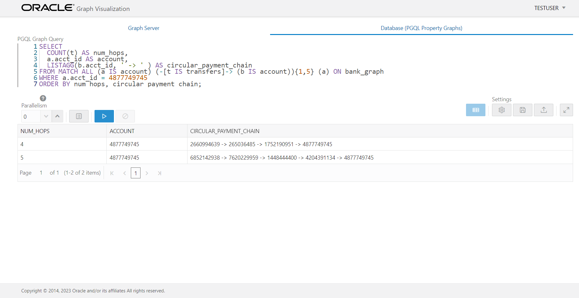
The next example of variable-length paths query looks for circular payment chains, meaning money transfers from one account via one or more intermediate accounts back to the same account.
---------------------------------------------------------------------
-- Another variable-length path query example:
--   Find all circular payment chains for a given account
---------------------------------------------------------------------
SELECT
  COUNT(t) AS num_hops,
  a.acct_id AS account,
  LISTAGG(b.acct_id, ' -> ' ) AS circular_payment_chain
FROM MATCH ALL (a IS account) (-[t IS transfers]-> (b IS account)){1,5} (a) ON bank_graph
WHERE a.acct_id = 4877749745
ORDER BY num_hops, circular_payment_chain;
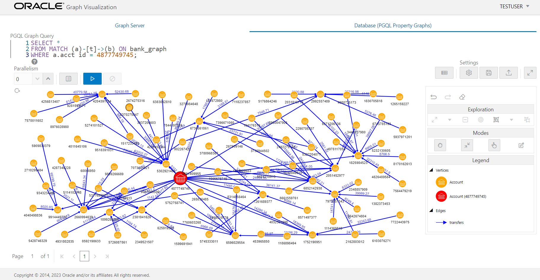
The result you can see in the following graphic captured from the Oracle Graph Visualization application. This web application is available as one of the clients tools previously mentioned or can be deployed on OCI via the Oracle Cloud MarketPlace.
It is up to you now to try out with the various capabilities of PGQL to query your graph.
You are also free to extend the underlying data set with new tables, such as for account holders, or new properties in the existing tables. Then you can create one or more alternative graphs that includes the changes.
Have fun!
Further reading
- Property Graph Query Language documentation
- Posts about Oracle Graph Technologies on Oracle Database Insider
- Analytics and TechCast Days Youtube channel with published videos including presentations about Graph Analytics
- Oracle Graph Learning Path
- Querying Graphs with SQL and PGQL: What are the differences?