 With the support of GraphQL queries in the new Oracle REST Data Services (ORDS) 23.3, another graph engine has been added to the Oracle Database. Due to different origins and approaches, is it better not to make a comparison with property graphs or RDF graphs or ontologies, or what exactly makes the engines so incomparable? Short examples will be used to show how the new GraphQL support works with ORDS 23.3 and where it can be used in comparison to property graphs in the Oracle Database.
The news in brief
Since the last post on GraphQL with WebLogic and the Google graphql API, with Spring or with Java Microprofile in 2021, a few things have happened. The number of GraphQL projects at companies in all sectors has increased significantly. Oracle’s open source framework Helidon is now available in Version 4 and, in addition to Java Microprofile 6 support, offers significantly better performance for REST services and therefore also for GraphQL. This is thanks to an even further optimized HTTP server “Nìma” (instead of Netty) and its support for virtual threads of JDK 21. The distributed Java InMemory database Coherence also supports virtual threads and is even more closely integrated with Helidon (and GraphQL).
Oracle Database 23c has integrated support for property graphs into the core of the database. This has been made possible by the addition of property graph queries to the SQL 2023 standard. Various graph database vendors have collaborated on this extension of the SQL standard. The Oracle database 23c is the first implementation in a commercial and open source database.SQL/PGQ is very similar to Oracle’s previous query language PGQL for property graphs.
The support for ontologies by storing and querying triplet information via W3C standard SPARQL, embedded in Oracle SQL functions, has been enhanced by better visualization tools and APEX plugins such as Graph Visualizer. In addition to RDF ontologies and SPARQL, this also supports the visualization of property graphs and queries via SQL/PGQ.
For REST services generated from database objects, Oracle REST Data Services (ORDS) Version 23.3 has recently made the GraphQL query language available. The ORDS container generates usable GraphQL structures from database objects during operation, without any programming. These can be tested and scripted immediately in the supplied browser-based “graphiql” interface.
Is there a winning standard that can do everything and will replace everything?
No. All three graph engines have their preferred field of application, their own origin and lasting benefits. They could each be embedded or bracketed together, for example with SQL means of a converged database that masters all standards… or ultimately they could be formulated as a super-generic world-describing ontology across everything.
![]() GraphQL has its origins and area of application in the development of REST services and is intended for backend developers. Various REST services and now also any data sources can be interconnected to form a comprehensive data model and service. Originally disjoint services and data can be brought into relation with each other and connected to form an “over-graph”. When a request is made, the GraphQL engine decides which of the available services actually need to be called and does so in parallel. This allows performance and the amount of data transferred to be optimized, known as “right-fetching”. The results of queries using GraphQL are always JSON tree structures whose attributes are either “scalars”, i.e. simple data types, or “objects”, subtypes or sub-graphs. In the latter case, the name of the attribute stands for a named relationship to a sub-graph. to break away a little from object-oriented tree models…
GraphQL has its origins and area of application in the development of REST services and is intended for backend developers. Various REST services and now also any data sources can be interconnected to form a comprehensive data model and service. Originally disjoint services and data can be brought into relation with each other and connected to form an “over-graph”. When a request is made, the GraphQL engine decides which of the available services actually need to be called and does so in parallel. This allows performance and the amount of data transferred to be optimized, known as “right-fetching”. The results of queries using GraphQL are always JSON tree structures whose attributes are either “scalars”, i.e. simple data types, or “objects”, subtypes or sub-graphs. In the latter case, the name of the attribute stands for a named relationship to a sub-graph. to break away a little from object-oriented tree models…
![]() PGQL and the SQL/PGQ contained in the SQL:2023 standard are, like GraphQL, able to define “over-graphs” on existing structures, but in this case only database structures such as tables and views. This means that any relationships can be freely named and defined and are no longer only visible as “master-detail”. The strength of SQL/PGQ lies in the analysis of metadata, complex relationships of information. Even deeply hierarchical or cyclical relationships can be resolved, the shortest paths with the fewest “hops” can be calculated or circular dependencies can be found, e.g. to uncover money laundering through triangular or polygonal postings. Further analyses of graphs are possible through the use of Graph Algorithmen and Graph Machine Learning, which are available via Graph Server. Further information can be found in the documentation.
PGQL and the SQL/PGQ contained in the SQL:2023 standard are, like GraphQL, able to define “over-graphs” on existing structures, but in this case only database structures such as tables and views. This means that any relationships can be freely named and defined and are no longer only visible as “master-detail”. The strength of SQL/PGQ lies in the analysis of metadata, complex relationships of information. Even deeply hierarchical or cyclical relationships can be resolved, the shortest paths with the fewest “hops” can be calculated or circular dependencies can be found, e.g. to uncover money laundering through triangular or polygonal postings. Further analyses of graphs are possible through the use of Graph Algorithmen and Graph Machine Learning, which are available via Graph Server. Further information can be found in the documentation.
 SPARQL is the query language for ontologies in RDF, OWL, Turtle exchange format (and others). Relationships and user data are merging, and a distinction is no longer made between data and metadata. I have personally used ontologies primarily for modelling and documenting more complex systems and for data lookup in standardized databases. Here, graph and relationship structures are usually not “flanged” to existing tables or REST services, but complete graphs with all elements are maintained, exchanged, attached or linked. And, very sensibly, relationships (the edges in a graph, the predicates in a triplet) can be standardized and can be accessed on the Internet in the form of vocabulary libraries. These libraries are themselves documented graphs that can be integrated into your own ontology. In this way, several relationship and format models can be accommodated simultaneously in one graph, e.g. a generic organisational vocabulary (memberOf, hasMember, etc.), an exhaustive set of medical terms, diagnoses, active ingredients (SNOMED CT) or technical vocabulary for building JSON Schema structure descriptions. And much, much more, both (IT) technical and subject-related.
Part 1: GraphQL
How to install it ?
First queries with GraphQL
Adding some more relations
Adding a relation to JSON documents
Adding a relation to external REST services
Visualisation of GraphQL graphs
Part 2: SQL/PGQ
Preparation
Defining a small graph
Simple queries
Queries on metadata
Visualisiation of property graphs
Teil 1: GraphQL
GraphQL witht Oracle Database – how to install it ?
A blog entry by Jeff Smith explains how to set up the new ORDS 23.3 with GraphQL support. In principal, the following steps are meaningful for first testing:
-
Download the latest version of ORDS (23.3 or higher).
-
Download and install GraalVM EE for JDK 17, NOT the OpenJDK or Oracle JDK, not the “regular” GraalVM.
-
Download and install JavaScript support for GraalVM: correct, the GraphQL engine is written in server-side JavaScript.
with free internet access to the GraalVM downloads, the “Graal Updater” may also download its components directly:
gu install js
Or in all other cases, select “JavaScript Runtime” on the GraalVM download page, download and install the file locally:
gu -L install js-installable-svm-svmee-java17-windows-amd64-22.3.1.jar (or other version number) - Link ORDS with an existing Oracle Database 19c or higher.
<graalvm_home>/bin/java -jar ords.war install
Now there are various questions to answer, e.g. all features must be installed and database user and connect information must be entered. Then:
<graalvm_home>/bin/java -jar ords.war serve
This starts the local ORDS server with default specifications on http port 8080.
- Create a database demo user and activate it for REST access.
If not already available, it is recommended to create the HR demo schema and then use it. The SQL scripts required to create the user with its tables can be found in the ORACLE_HOME of your database in the subdirectory /demo/schema/human_resources, or for a few years now also on github for download.
Please use a privileged user such as SYS or SYSTEM and a tool of your choice, e.g. SQLcl or SQL*Plus.
Once the user has been created, you can also activate it for REST access as well as for the browser tool “SQL Developer Web” or the “Database Actions” tool palette with the following SQL.
BEGIN
	ORDS.ENABLE_SCHEMA(p_enabled => TRUE,
	                   p_schema =>'HR');
END;
/
- Now activate the HR demo tables for REST access.
We will add views and a JSON table later to deepen the features. For now, the user “HR” under SQL*Plus or SQLcl is sufficient:BEGIN ORDS.enable_object ( p_schema => 'HR', p_object => 'EMPLOYEES', p_object_alias => 'employees'); ORDS.enable_object ( p_schema => 'HR', p_object => 'DEPARTMENTS', p_object_alias => 'departments'); ORDS.enable_object ( p_schema => 'HR', p_object => 'LOCATIONS', p_object_alias => 'locations'); COMMIT; END; /
- Please start the ORDS container now. It generates a GraphQL data structure from the published tables and views at startup and keeps it in the cache for 8-24 hours (default parameter).
The ORDS parameters cache.metadata.graphql.expireAfterAccess and cache.metadata.graphql.expireAfterWrite can also be set to a few minutes, purely for test purposes, so that the ORDS is not permanently burdened with the creation of GraphQL structures.
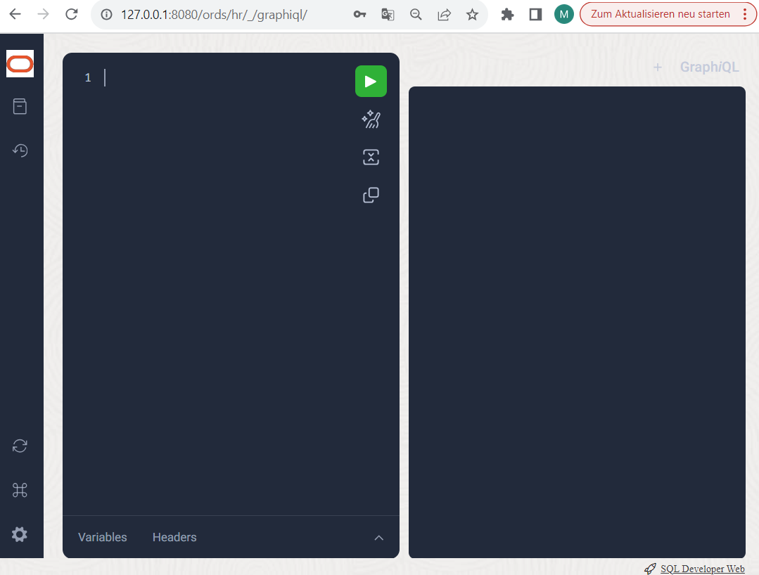
- Call up the GraphQL app “Graphiql” and formulate the first queries. With a browser of your choice, a call to the URL http://127.0.0.1:8080/ords/hr/_/graphiql/
should take you to the “graphiql” interface, with which you can view and query the objects as user “HR” that have just been released for REST access:
- Congratulations! Installation and initial setup are complete, let’s get down to business and see what’s possible here.
First queries with GraphQL
First click on the “Documentation Explorer” icon on the left-hand side of the window to display which data types ORDS read out at the start.
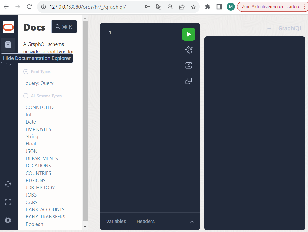
Only a Query is offered here as a “root type”. Other possible root types in GraphQL such as Mutation (data change) and Subscription (“subscription” or notification of changes) are not yet supported. However, the queries already have a lot to offer and provide a number of features that would otherwise require extensive programming. We will take a closer look at this in a moment.
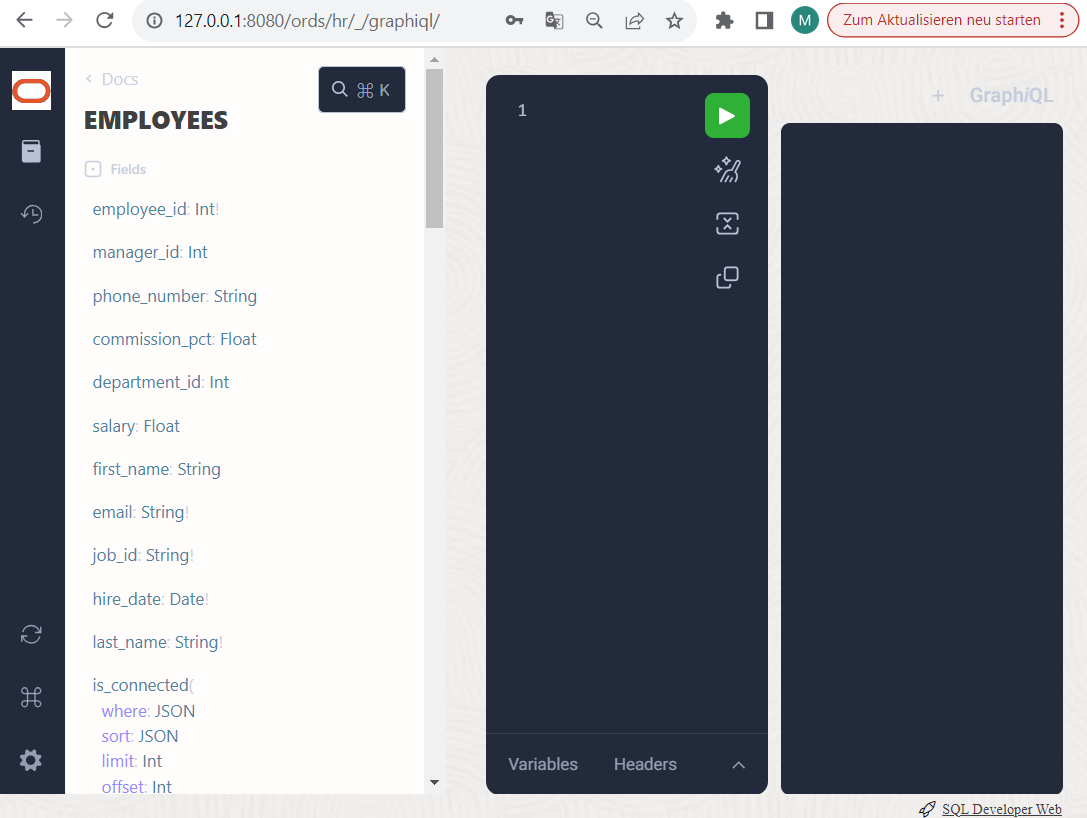
In our example environment, there are already significantly more schema types available than you will probably see. In addition to some “scalar” data types such as String, Int, Date, Float, Boolean etc., you should have some “object” data types such as DEPARTMENTS, EMPLOYEES and LOCATIONS. The data types are clickable and offer a description of their structure, i.e. on the one hand attributes with scalar data types behind them or on the other hand relationship attributes that refer to subtypes.
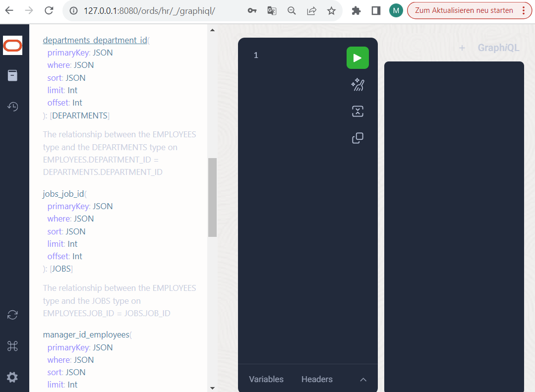
For example, EMPLOYEES have a directed relationship to DEPARTMENTS via the relationship attribute “departments_departments_id”. This attribute was automatically generated from the name of the underlying target table and the name of the primary key there. These are not yet very descriptive names for relationships, but we can help ourselves in further examples using database views. But that later.
As you can also see, relationship types always offer the option of filtering, sorting, limiting or even “paginating” data, i.e. skipping page by page by specifying sort+offset+limit. Let’s start with a simple query on the initial object EMPLOYEES to generate a tree structure.
In the query field, type the term “query” next to the “1”, followed by the desired name of your query (“myFirstQuery“) and a curly bracket. graphiql will then help you to select the desired attributes and relationships by entering the key combination <CTRL>+<SPACE>.
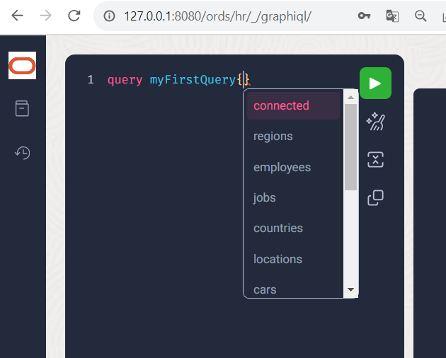
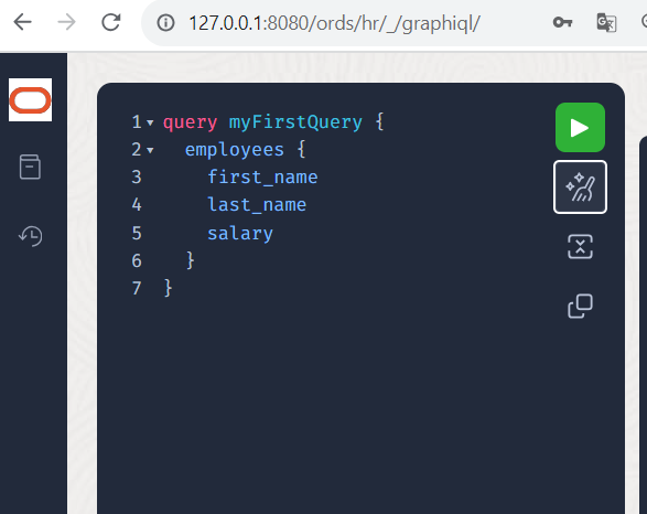
Now select the query attribute “employees” (a relationship to all objects of type EMPLOYEES), followed by a curly bracket. Within the curly bracket, press the key combination <CTRL>+<SPACE> again so that you select the attributes first_name last_name salary (separated by a space or comma). Then click boldly on the “broom” symbol (Prettify Query) and your query will be formatted nicely.
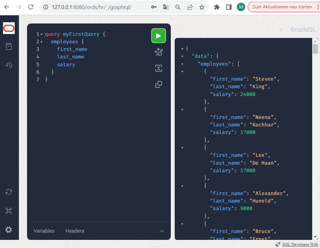
Now click on the green and white arrow symbol and execute the query.
Now play a little with filters and sorting. Add a round bracket immediately after the “employees” attribute, then enter <CTRL>+<SPACE> again to select a where condition and specify a JSON syntax (unfortunately without help this time) like this:

The filters can also be applied to the respective relationship types or subqueries. The syntax for where filters is very comprehensive and can be very complexly nested; you can find a more comprehensive description in the ORDS documentation. You can find one or two further examples in the blog entries by Jeff Smith, our ORDS “pope”.
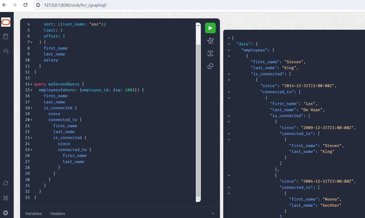
A more comprehensive example with sorting, filtering and pagination could look like this. Please note that the sorting criteria are packed into an array “[]” because there could be several criteria.
employees(where: {first_name: {eq: "Steven"}},
sort: [{last_name: "asc"}],
limit: 1
offset: 1 ) {
first_name
last_name
salary
}
}
Creating and attaching a new relation
Any other relationships with more descriptive relationship names but also with arbitrarily complex logic for determining the relationship can be created via relational views. So-called N:M relationship tables are usually used to temporarily store additional attributes or to create a “mapping” between source nodes and target nodes. If, for example, it is not just a hierarchical representation of which manager forms a department with which employees, but rather which of the employees know each other personally, the following approach might be useful. First of all, presented as a script and implemented in the “HR” schema:
INSERT INTO FACEBOOK (from_id, to_id, since) values (102, 100, to_date('01.01.2010'));
INSERT INTO FACEBOOK (from_id, to_id, since) values (100, 102, to_date('01.01.2015'));
INSERT INTO FACEBOOK (from_id, to_id, since) values (102, 101, to_date('01.01.2005'));
INSERT INTO FACEBOOK (from_id, to_id, since) values (101, 100, to_date('01.01.1999'));
COMMIT;
CREATE VIEW CONNECTED ("IS", "TO", SINCE) AS SELECT FROM_ID, TO_ID, SINCE FROM FACEBOOK;
ALTER VIEW CONNECTED
ADD CONSTRAINT FROM_FK FOREIGN KEY ( "IS" )
REFERENCES HR.EMPLOYEES ( EMPLOYEE_ID ) DISABLE ;
ALTER VIEW CONNECTED
ADD CONSTRAINT TO_FK FOREIGN KEY ( "TO" )
REFERENCES HR.EMPLOYEES ( EMPLOYEE_ID ) DISABLE ;
BEGIN
ORDS.enable_object ( p_schema => 'HR', p_object => 'CONNECTED', p_object_type => 'VIEW', p_object_alias => 'connected');
END;
To explain: we first create a “FACEBOOK” table and enter which person actively knows other people and for how long.
Now we create a view above it with more descriptive names for the later GraphQL query. And we create two relational relationships between FACEBOOK and EMPLOYEES. However, these are deactivated and should have no effect, they only serve to ensure that the GraphQL engine recognizes these relationships and creates relationship types. Any other relationships in the base table “FACEBOOK” remain unaffected. Only the CONNECTED view is enabled for access via GraphQL, the FACEBOOK table should remain hidden.
Please start the ORDS container first so that the new addition to the data model is also recognized. Then reread the schema in graphiql by clicking on the refetch symbol at the bottom left of the screen.
Now you can display and query the free relationship between the employees and the “who-knows-who” in GraphQL. To do this, create a second query and go through the hierarchy a little: The employee with the ID 100 has which name and knows which other persons and since when?
employees(where: {employee_id: {eq: 100}}) {
first_name
last_name
is_connected {
since
connected_to {
first_name
last_name
}
}
}
}
To execute the query, you can select from a list of defined “named” queries by clicking on the green button:
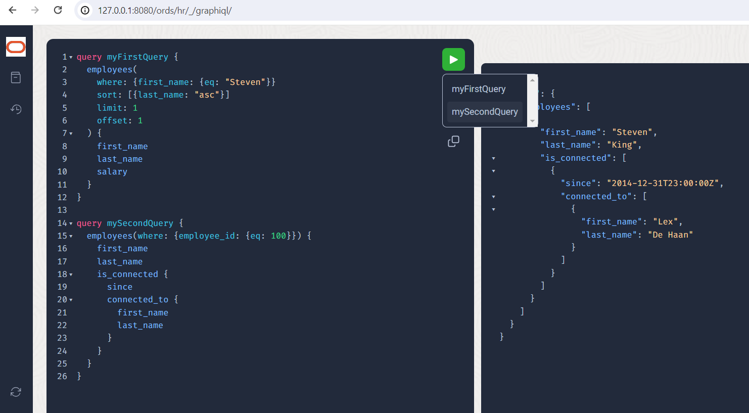
Let’s move on to a deliberate limitation of the nesting depth in order to avoid deep-cyclic queries and perhaps avert DoS attacks. Who does Mr. King know, and who do these people know?
Look, Mr. King knows Mr. De Haan, and he also knows Mr. King, but from a different time.
Let’s filter out these relationship data and see how deeply we could link them here:
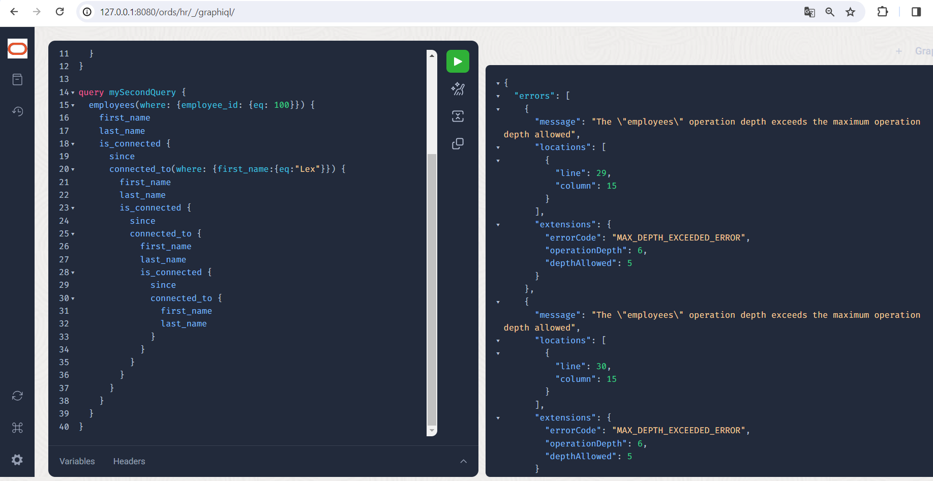
Unfortunately we don’t get very far, we get the error message “MAX_DEPTH_EXCEEDED_ERROR”. By default, queries may not recurse deeper than 5 levels: employees->is_connected->connected_to->is_connected->connected_to are 5 “hops”, so to speak. However, this limit can be shifted using a parameter in the configuration file pools.xml or settings.xml. The parameter for this is feature.grahpql.max.nesting.depth and is of course documented.
At this point it should be mentioned that SQL/PGQ could really come into its own here. Queries on the relationship or recursion depth and relationship metadata are possible, even without having to specify each individual relationship type. For example, a query of the type “Show how many hops employee A has with B, sort by the number of hops” determines the direct and indirect acquaintances, the shortest path between two people. This will be discussed later in part 2 about SQL/PGQ.
Defiing a relation to JSON documents
GraphQL was intended to establish relationships between REST services and the resulting data. A higher-level data model, a graph, describes the entire data structure across all relevant services. If a GraphQL query is sent to a relationship type, a so-called “resolver” is called in the GraphQL server. This is a piece of code, a bit of logic, which retrieves the data for the requested data type in any way that is usually still to be programmed and prepares it (as little as possible). In ORDS, there is no need to program these resolvers manually, because ORDS comes with its own resolvers, which generate GraphQL structures (stored via “SDL”, Schema Definition Language) from published database tables and views and read out or integrate these database structures. But thanks to the Oracle “converged database” features, tables and views could refer to JSON documents via REST calls (modern example: calling a generative AI with additional information, e.g. on the “locations” of employees) or contain and manage them directly. And all of this securely and with high performance – try it out!
So let’s first create a JSON key-value table, also called a “collection” in the SODA and MongoDB API. I am using the SODA API here for convenience, it could also have been a table created with pure SQL with a JSON column. Please run the following SQL as HR user again:
DECLARE
    collection  SODA_Collection_T;
    metadata VARCHAR2(4000) :=
      '{"keyColumn" : {"name" : "ID",  "assignmentMethod": "UUID" },
        "contentColumn" : { "name" : "DATA", "sqlType": "BLOB" } }';
    doc1  SODA_DOCUMENT_T;
    doc2  SODA_DOCUMENT_T;
    doc3  SODA_DOCUMENT_T;
    status number;
BEGIN
    collection := DBMS_SODA.create_collection('CompanyCars', metadata);
    doc1 := SODA_DOCUMENT_T(b_content => utl_raw.cast_to_raw('{"licensePlate":"M-P-1234","vendor":"Skoda","model":"Kodiaq","fuel":"Diesel","gearbox":"automatic","displacement":"2.0l","leaseStart":"2017-01-06","leaseEnd":"2019-01-15","employeeID":102}'));
    doc2 := SODA_DOCUMENT_T(b_content => utl_raw.cast_to_raw('{"licensePlate":"M-O-7182","vendor":"Peugeot","model":"5008","fuel":"Diesel","gearbox":"automatic","displacement":"2.0l","leaseStart":"2019-01-16","leaseEnd":"2023-01-15","employeeID":102}'));
    doc3 := SODA_DOCUMENT_T(b_content => utl_raw.cast_to_raw('{"licensePlate":"M-B-5678","vendor":"Mini","model":"Countryman","fuel":"Benzin","gearbox":"automatic","displacement":"1.8l","leaseStart":"2023-01-16","leaseEnd":"2026-01-16","employeeID":100}'));
    status := collection.insert_one(doc1);
    status := collection.insert_one(doc2);
    status := collection.insert_one(doc3);
END;
/
We now place a more descriptive view “CARS” on top, link it to the employees table “Employees” using a foreign key and publish the view for REST access and for GraphQL:
CREATE OR REPLACE VIEW CARS AS
select id, json_value(data, '$.employeeID' returning number) owned,
           json_value(data, '$.model' ) model,
           json_value(data, '$.vendor' ) vendor,
           json_value(data, '$.licensePlate' ) licensePlate,
           json_value(data, '$.displacement' ) displacement,
           json_value(data, '$.leaseStart' returning date ) leaseStart,
           json_value(data, '$.leaseEnd' returning date ) leaseEnd
from "CompanyCars" ;
/

ALTER VIEW CARS
    ADD CONSTRAINT CARS_EMP_FK FOREIGN KEY ( owned ) REFERENCES EMPLOYEES ( EMPLOYEE_ID ) DISABLE ;
/

ALTER VIEW CARS
    ADD CONSTRAINT CARS_PK PRIMARY KEY (id) DISABLE;
/

BEGIN
 ORDS.enable_object (p_schema => 'HR', p_object => 'CARS', p_object_type => 'VIEW', p_object_alias => 'cars');
END;
/
Please start the ORDS container first so that the new addition to the data model is recognized more quickly. Then reread the schema in graphiql by clicking on the refetch symbol at the bottom left of the screen.
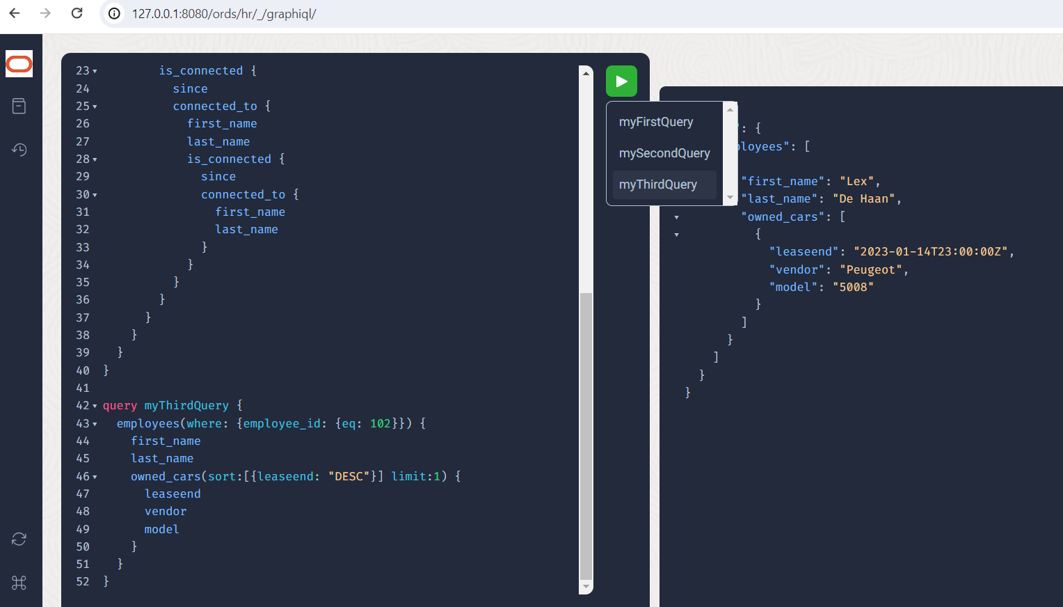
Now you can easily list which company vehicles the employee with ID 102 owned or, even better, which company vehicle he currently owns.
A small bug: with sort and where entries, the database objects queried must not have “lowercase” or “MixedCase” designations. Usually, only capitalized names are used in the database anyway.
Also note: limit specifications ideally require a primary key on the queried object, otherwise the internal ROWID column is used. And this does not exist for views, only for tables.
query myThirdQuery {
  employees(where: {employee_id: {eq: 102}}) {
    first_name
    last_name
    owned_cars(sort:[{leaseend: "DESC"}]
               limit:1) {
      leaseend
      vendor
      model
    }
  }
}
The result should look like this:
Of course, we are not forced to enter the graph only via the employees. For example, we could also retain the depth limit for recursions by starting the query at a lower level. A list of all company vehicles with their owners would be possible using the following query:
query myFourthQuery {
  cars {
    vendor
    model
    displacement
    cars_owned {
      first_name
      last_name
    }
  }
}
Defining a relation to a REST service
Traditionally, custom resolvers are programmed in Java or JavaScript that call remote REST services to incorporate their data and logic. Here, however, we can use the existing resolvers contained in ORDS within the Oracle Database to achieve the same goal via views and function calls. In our example, we would like to enrich the vehicle data a little with additional information about the model and a link to the image of the respective vehicle type. To do this, we wrap a REST service call in a function, integrate it into a view and relate it to the existing “CompanyCars” JSON table via a foreign key.
The procedure is always the same: a view that does arbitrarily complex things and thus implements a complex relationship to other objects is related to other objects via foreign keys. Incidentally, this works quite similarly with SQL/PGQ.
Let’s start by giving our “HR” user the authorization to access a REST service of the Wikipedia library. As a privileged user, e.g. “SYS“, please add the public Wikipedia library to an ACL list for HTTP access:
BEGIN
    DBMS_NETWORK_ACL_ADMIN.APPEND_HOST_ACE(
        host => 'en.wikipedia.org',
        ace  =>  xs$ace_type(
            privilege_list => xs$name_list('http'),
            principal_name => 'HR',
            principal_type => xs_acl.ptype_db
        )
    );
END;
/
Now, as user HR, we create a function that calls the REST service and a view that is later limited in GraphQL by a WHERE clause so that not all vehicle data of all vehicles is always retrieved. The function could also have been written in JavaScript in version 23c, but I didn’t want to get too verbose:
CREATE OR REPLACE FUNCTION CARDETAILS( brand_model in varchar2) return varchar2
AS
    l_url             VARCHAR2(400) := 'https://en.wikipedia.org/api/rest_v1/page/summary/';
    req               utl_http.req;
    resp              utl_http.resp;
    buffer            VARCHAR2(32767);
BEGIN
   l_url := l_url || brand_model;
   -- in case you are behind a proxy, please uncomment the following line after setting the correct proxy address
   -- utl_http.set_proxy('http://username:passwd@192.168.22.33:5678');
   req := utl_http.begin_request(url => l_url, method => 'GET');
   utl_http.set_header(req, 'Accept', 'application/json');
   resp := utl_http.get_response(req);
   BEGIN
      utl_http.read_text(resp, buffer);
   EXCEPTION
      WHEN utl_http.end_of_body THEN
         utl_http.end_response(resp);
   END;
   return buffer;
END;
/

CREATE OR REPLACE VIEW CARINFO AS SELECT
                       id AS avail,
                       json_value(cardetails(vendor||'_'||model), '$.extract') extract,
                       json_value(cardetails(vendor||'_'||model), '$.thumbnail.source') image
FROM CARS;
/

ALTER VIEW CARINFO ADD CONSTRAINT carinfo_car_fk FOREIGN KEY (avail) REFERENCES CARS (id) DISABLE;
/

BEGIN
  ORDS.enable_object (p_schema => 'HR', p_object => 'CARINFO', p_object_type => 'VIEW', p_object_alias => 'carinfo');
END;
/
Please start the ORDS container first so that the new addition to the data model is recognized more quickly. Then reread the schema in graphiql by clicking on the refetch symbol at the bottom left of the screen.
Now you can call up a short description and a picture for each company vehicle that is also entered on Wikipedia. Please note that for reasons of simplicity, the REST service is called several times, albeit in parallel and not serially. Nevertheless, you should think about a better result structure in “real life”, e.g. the called function could rather become a pipelined function and return the elements of the JSON result as columns, or something could be done with the fairly new SQL macros.
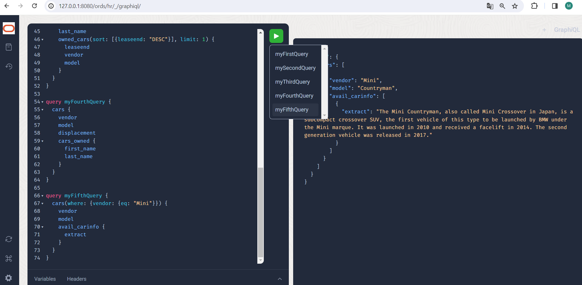
Please also note that error messages may occur for the same reason if you query several attributes from the CARINFO view: Too many simultaneous HTTP requests from the database are warned. However, the following GraphQL query on an attribute should also work for you:
query myFifthQuery {
  cars(where: {vendor: {eq: "Mini"}}) {
    vendor
    model
    avail_carinfo {
      extract
    }
  }
}
So much for the basic features and principles of GraphQL within ORDS. If you have any further wishes or ideas about what else could be included, our Jeff Smith is looking forward to your feedback and input! Personally, I think the Query support is already very successful, even if I wish I could name relationships freely. Views can be used for many things. Direct support for JSON data types and JSON Duality Views would help a lot, currently fields of type JSON are rendered as MIME-encoded content. I would very much like to see mutations and subscriptions, the former would harmonize very nicely with JSON Duality Views and the latter could be implemented as continuous queries, as long as they don’t get too complex. GraphQL support for variables and fragments is provided here because it is independent of the other implementation and resolvers.
Visualising GraphQL Graphs
Displaying and evaluating the results from GraphQL queries is easy with analysis tools such as Oracle Analytics Cloud or Analytics Server. Oracle Analytics accepts REST services as data sources and can handle data in JSON structures. Complex JSON structures with deep nesting are now permitted; the REST service called, in our case GraphQL in the ORDS container, does not necessarily have to be bound to the ODATA JSON format – both variants are supported.
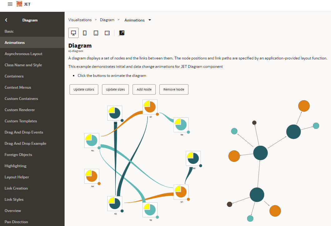
The particularly comprehensive open source framework Oracle JET (JavaScript Extension Toolkit) offers a visualization of graphs that can be adapted down to the last detail. This visualization bears the simple name “Diagram” and is completely customizable in terms of node display and content, animations and colors, drag & drop events and much more. TypeScript knowledge and knowledge of JavaScript frameworks for data preparation are necessary here, but certainly worthwhile.
If a graphical representation of the graph structure or metadata is required, the first appealing interfaces are now available. It was not GraphQL’s forte to analyze relationships and links, but rather to define relationships and resolve them optimally and efficiently. One appealing tool, for example, is GraphQL Voyager. It prepares a GraphQL metadata query that outputs all structures and components as a result. The result is then copied into the tool and the data structures and relationships can be visualized and scrutinized.
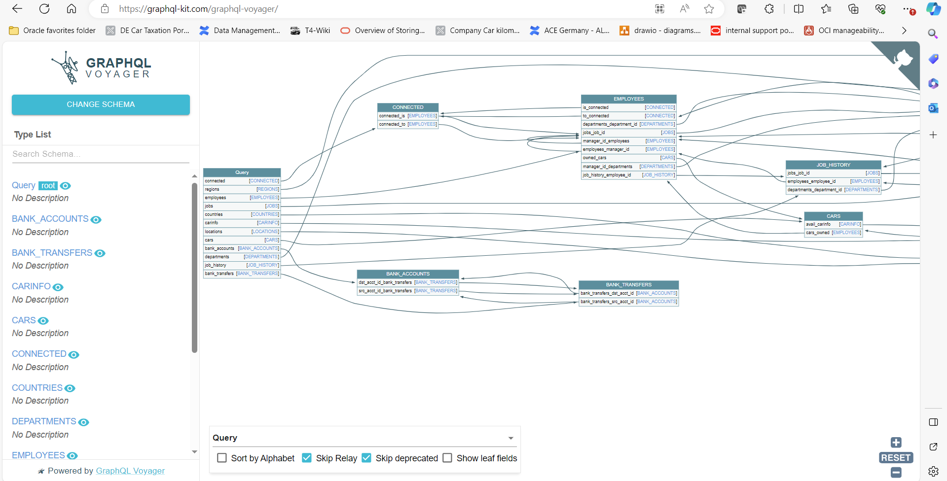
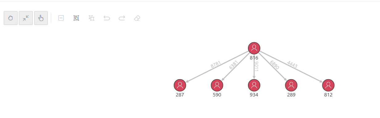
Here you can see very clearly that a GraphQL query could start at any node of the graph (employees, cars,…) and how to navigate from there to the other linked nodes. If you are more interested in displaying the result data of a GraphQL query as a graph, this tool could be interesting: the jsonCrack JSON Editor
Although it only displays the structures that were queried in a GraphQL query, it shows nodes and data very nicely if a “graph” is selected instead of the standard “tree” display.

The possibilities for visualization and also embellishment of the display are understandably much more comprehensive with SQL/PGQ graphs. Let’s now take a brief look at the SQL/PGQ graphs for comparison. By the way, you can find an even better insight into SQL/PGQ in a recent blog entry by my dear colleague Karin Patenge.
Part 2: SQL/PGQ
Let’s now make a brief comparison with SQL/PGQ to show its strengths. We have already loaded data for querying in part 1, so we just need to overlay a graph and formulate the kind of queries that are rather difficult to implement in GraphQL. Or almost, anyway. Because such a property graph only likes tables and materialized views as the basis for its vertices and edges, not views. So we first have to turn the “CARS” view into a materialized view (preferably with automatic refresh) or enrich the “CompanyCars” table with some columns that are needed as primary and foreign keys. I have opted for the materialized view. Please run the following SQL as HR user:
create materialized view cars_mv as
select     json_value(json_document, '$.employeeID' returning number) empid,
           json_value(json_document, '$.model' returning varchar2(50)) model,
           json_value(json_document, '$.vendor' returning varchar2(100)) vendor,
           json_value(json_document, '$.licensePlate' returning varchar2(100)) licensePlate,
           json_value(json_document, '$.displacement' returning varchar2(10)) displacement,
           json_value(json_document, '$.leaseStart' returning date ) leaseStart,
           json_value(json_document, '$.leaseEnd' returning date ) leaseEnd
from "CompanyCars" ;
/
The CARINFO view would also have to be materialized, i.e. all data from REST calls to Wikipedia for the vehicles in question would have to be stored temporarily and updated from time to time. SQL/PGQ is primarily suitable for analyses, and these should be as fast as possible. Let’s dispense with this part because I think the purpose and benefits are clear.
Defining a graph on top of an existing data model
With GraphQL, published tables, views and their foreign keys are used for REST access to generate a graph. Its documentation is available as an SDL (Schema Definition Language) document and can be accessed via REST. For the creation of property graphs, there is an SQL/PGQ syntax that defines the base tables for nodes and edges/relationships and can give the relationships their own names. This information is stored in internal database tables and used in queries to turn SQL/PGQ syntax into more or less complex SQL queries. Please run the following command with an SQL tool such as SQLcl, Jupyter Notebook or SQL*Developer against your Oracle database, as always as user HR. If you are using Oracle 23c as your database, the SQL/PGQ parser is integrated and you can use any tool. Otherwise, the PGQL parser usually included in the tool is used, which may still have slight differences to SQL/PGQ. The tool should therefore be as up-to-date as possible in order to cover all SQL/PGQ features.
CREATE PROPERTY GRAPH employee_network
  VERTEX TABLES(
    employees
      KEY ( employee_id )
      PROPERTIES all columns
      LABEL employee,
    cars_mv
      KEY ( empid, licenseplate )
      PROPERTIES all columns
      LABEL cars
  )
  EDGE TABLES(
    facebook as connected
      key (from_id, to_id)
      SOURCE KEY ( from_id ) REFERENCES employees (employee_id)
      DESTINATION KEY ( to_id ) REFERENCES employees (employee_id)
      PROPERTIES (since),
    cars_mv as owned
      key (empid, licenseplate)
      SOURCE KEY ( empid ) REFERENCES employees ( employee_id )
      DESTINATION KEY ( empid, licenseplate ) REFERENCES cars_mv ( empid, licenseplate )
  );
/
Simple queries
The nodes EMPLOYEE and CARS as well as the edges/relationships CONNECTED and OWNED are available through the graph just defined.The data or keys of the OWNED relationship are immediately available in the node table CARS_MV; due to the existing 1:N relationship, no N:M relationship table was used.
With the help of SQL/PGQ, we can now choose which relationship (OWNED) and in which direction (->) we want to find out which company vehicles the employee with ID 102 owned.
select *
from   graph_table (employee_network
         match
         (e is employee) - [is owned] -> (o is cars)
         where e.employee_id = 102
         columns (e.employee_id as owner_id,
                  o.model as model,
                  o.vendor as vendor)
       )
order by 1;
Result:
OWNER_ID    MODEL    VENDOR
102         Kodiaq   Skoda
102         5008     Peugeot
To find out which persons the employee with ID 100 knows directly, as in GraphQL, the following query can be used.
The CONNECTED relationship may also have attributes that can be queried:
select *
from   graph_table (employee_network
         match
         (e1 is employee) - [c is connected] -> (e2 is employee)
         where e1.employee_id = 102
         columns (e1.first_name as is_first_name,
                  e1.last_name as is_last_name,
                  e2.first_name as knows_first_name,
                  e2.last_name as knows_last_name,
                  c.since as since,
                  e2.employee_id as knows_id)
       )
order by 1;
Result:
IS_FIRST_NAME    IS_LAST_NAME    KNOWS_FIRST_NAME    KNOWS_LAST_NAME    SINCE                  KNOWS_ID
Lex              De Haan         Neena               Kochhar            2005-01-01 00:00:00    101
Lex              De Haan         Steven              King               2010-01-01 00:00:00    100
Queries on metadata
Now we come to the particular strengths of SQL/PGQ.
If it is unknown via which relationships or via how many hops or recursions a node is connected to another node, we do not have to manually click our way through a path/tree structure, but can simply omit certain details such as paths, or we can determine the maximum recursion depth ourselves and in short form. For example, to check whether someone has been connected directly to themselves (by mistake?), you could formulate the following query:
select *
from   graph_table (employee_network
         match
         (p1 is employees) - [is connected] -> (p1)
         columns (p1.employee_id as from_id,
                  p1.first_name as first_name,
                  p1.last_name as last_name,
                  p1.employee_id as to_id)
       )
order by 1;
The result set should be empty here, nothing found.
But this should be the case around two corners, as we also discovered in GraphQL – here is the equivalent in SQL/PGQ with a number of hops:
select *
from   graph_table (employee_network
         match
         (p1 is employees) - [is connected] -> {2}(p1)
         columns (p1.employee_id as from_id,
                  p1.first_name as first_name,
                  p1.last_name as last_name)
       )
order by 1;
The result says yes, that applies to both Mr. De Haan and Mr. King:
FROM_ID  FIRST_NAME  LAST_NAME
100      Steven      King
102      Lex         De Haan
A small note: if no result is returned when specifying a quantification or number of hops, you are probably using a tool with a somewhat outdated integrated PGQL parser that ignores this information. This is the case with the “Database Actions” tool contained in ORDS 23.3. If you are working with an Oracle Database 23c, you can bypass the parser in the tool by wrapping the SQL/PGQ query in a view and then retrieving the view. Otherwise, upgrading or changing your tool will help. There are separate PGQL parsers available for download that can be integrated into SQLcl, for example.
Now a short “ranking” query: which employees know themselves via any kind of relationship and with as few hops as possible, a maximum of 3 hops are allowed?
select from_id, first_name, last_name, count(1) as num_hops
from   graph_table (employee_network
         match
         (p1 is employees) - [] -> {1,3}(p1)
         columns (p1.employee_id as from_id,
                  p1.first_name as first_name,
                  p1.last_name as last_name)
       )
group by from_id, first_name, last_name order by num_hops;
Result:
FROM_ID FIRST_NAME LAST_NAME NUM_HOPS
101     Neena      Kochhar   1
100     Steven     King      2
102     Lex        De Haan   2
This example should show a little of how to use SQL/PGQ. The scenario used may be rather trivial, but please imagine that the queries are not about people but about bank accounts, and you have just found triangle postings to perform tax evasion or money laundering… and exactly this kind of example with a few more queries can be found on an example repository for PGQL (and also SQL/PGQ) on github. There you will also find further examples that use the prepared property graph algorithms mentioned at the beginning, which can be used in the separately downloadable Graph Server.
Visualising Property Graphs
Of course, the purely relational result data from SQL/PGQ queries can be prepared in any analysis tool, just as with GraphQL queries in the Oracle Analytics Cloud or the Analytics Server. There are also several plugins and tools that are specifically dedicated to displaying property graphs:
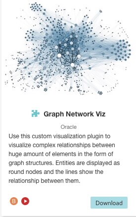
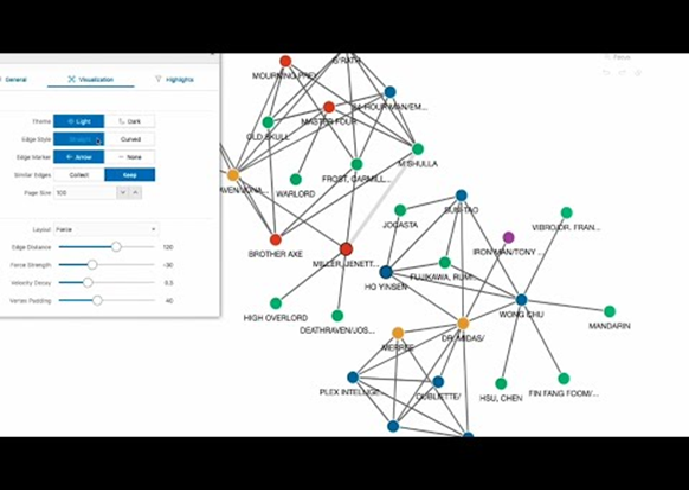
The Oracle Analytics Cloud Plugin “Graph Network Viz” or just called Property Graph Plugin can be installed later via the Oracle Analytics Extension Library. You can find a more detailed description of how to set it up in our Analytics colleagues’ blog. The plugin offers some standard analyses on property graphs, for example Shortest Path or Node Ranking, without an additional graph server.
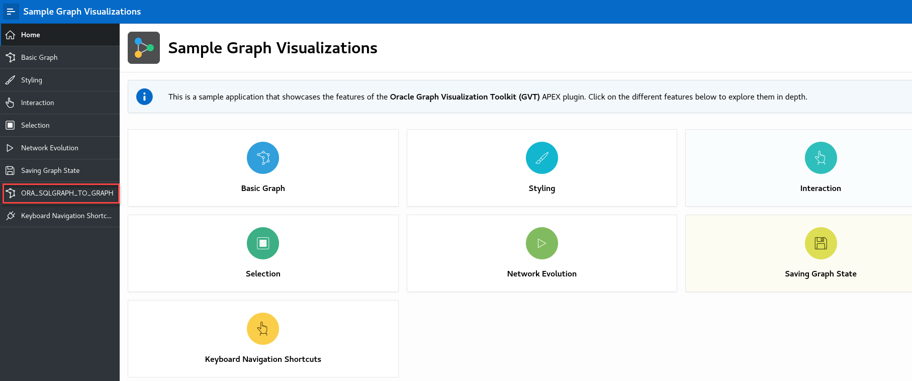
The “Graph Visualization Application” user interface contained in the separately downloadable Graph Server visualizes SQL/PGQ queries as graphs. Numerous customizations of the display are possible and documented. A short YouTube video shows what this could look like.
A Property Graph plugin for Jupyter Notebooks enables working with graphs such as creating, loading and querying, but also simple visualizations can be created.
A new plugin for Application Express (APEX), called Graph Visualization, is still in preview status, but it can already be seen that it will offer many customization options. It can of course already be integrated into your APEX environment, as it is available for download in the APEX GitHub repository. You can find brief instructions on how to integrate it in the Developer’s Guide for Property Graphs.
The Autonomous Database in the Oracle Cloud Infrastructure in the Autonomous Warehouse and Autonomous Transaction Processing versions comes with the very comprehensive Graph Studio tool to manage property graphs and RDF graphs and to visualize queries comprehensively. Graph Studio is originally based on the Graph Visualization Application and the Jupyter Notebook plugin, which extends this tool considerably.
Sum up
Different graph standards have their own application purpose. If SQL/PGQ is used more for analyzing complex linked data, GraphQL can be used to link originally disjoint data sources and call or query them in such a way that only the required data is retrieved and only the necessary backend services are triggered. The automatic generation of GraphQL structures and filters from relational data simplifies the provision of GraphQL graphs. The automatism can also be used to integrate external data sources and REST services into the generated graphs, offering a good introduction for database developers to the world of GraphQL and certainly more than that.
Links
PGQL Spec Site (just for completeness)
GraphQL with ORDS 23.3 documentation
SQL/PGQ with Database 23c documentation
Ideas and improvement suggestions on GraphQL support to Jeff Smith
Database 23c SQL/PGQ examples on github