
Leo Li — AI Infrastructure Architect, JAPAC Center of Excellence (CoE)
Natarajan Marimuthu — Master Principal Cloud Architect
Ussama Muhammad — Principal Cloud Architect, Cloud Engineering ASEAN
Durga Prasad Paladugula — Contractor
Many customers already have data pipelines that work well. The challenge is finding a way to run them where the data needs to stay, or close enough to its source for the application to respond quickly. Some use cases have data residency requirements that restrict raw data from leaving the customer’s security boundary. Others benefit from local processing to reduce data-transfer delays. You may have either requirement, or both.
The architecture brings existing extract, transform, and load (ETL) pipelines and machine learning operations (MLOps) workflows to Oracle infrastructure at the customer site. Oracle Autonomous AI Database (ADB) supports scheduling and access to published results. The pipeline itself runs in the local execution environment. In this design, raw inputs and intermediate processing stay local, while a customer-defined publication policy governs what is sent to cloud services.
In this post we:
- Show a local execution pattern for data residency–sensitive use cases, low-latency applications, or both.
- Explain how a solution built with ADB scheduling, a local execution service, and controlled publication connects pipelines to analytics.
- Describe two levels of optimization and interpret recorded proof-of-concept observations, including their test conditions and measurement scope.
Background
A typical operational pipeline starts by reading, cleaning, and aggregating source data. The next stages may prepare features, train models, generate forecasts, and detect anomalies. Operations teams use these outputs through dashboards and applications to understand what is happening and decide where to act.
These stages use infrastructure in different ways. ETL can be heavy on CPU, memory, and storage bandwidth. Model processing may use a graphics processing unit (GPU), while combining predictions and applying detection rules brings work back to the CPU. Matching resources to these stages gives us room to improve how the pipeline runs.
Where the pipeline runs also matters. If raw data cannot leave the customer boundary, processing needs to happen there. If the application needs a quick response, placing ETL near data generation can reduce the delay of transferring raw inputs to a remote environment. That can help applications that support mission-critical operations and real-time decisions.
Either reason can make local processing useful. Optimization then helps the pipeline run more efficiently in that environment. The overall application response also includes how data arrives, when processing starts, and how the result is used.
Oracle Roving Edge Infrastructure and Oracle Compute Cloud@Customer offer ways to bring Oracle compute and storage services to the customer site. Which option fits will depend on the workload, capacity, supported configuration, and how you plan to operate it. They are deployment options in this architecture. The observations below do not establish performance for a specific RED generation or Compute Cloud@Customer configuration. [1, 2]
Technical architecture
Figure 1 shows the two parts of the design. In the customer data center, local storage holds raw inputs, intermediate datasets, and model artifacts, and an execution engine runs the pipeline. In an Oracle Cloud Infrastructure (OCI) region, solution tables in ADB hold permitted pipeline metadata and run history. Selected outputs pass through a publication step to OCI Object Storage for ADB access.
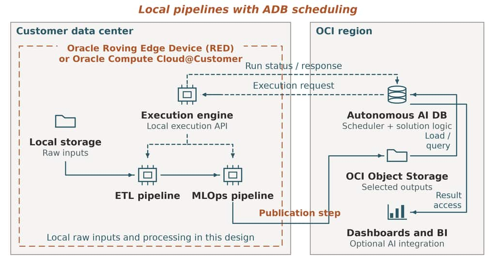
Figure 1. Logical deployment pattern for local pipelines with ADB scheduling and result access. Requests and status travel in separate directions. Selected outputs are published to OCI Object Storage for ADB access. The depicted residency boundary depends on configuration, connectivity, access controls, and the customer’s publication policy. Supporting network services are omitted.
Figure 1 shows three key ideas:
- Local execution: storage, ETL, MLOps, and the execution engine share the customer environment. The design places raw-data processing within that environment and near its source.
- Database-supported automation: solution components use Oracle APEX and ADB to manage definitions, schedules, and run history. A custom local service receives requests and reports progress and completion.
- Controlled publication: a separate solution component selects outputs for cloud access. The customer policy applies to derived data and model artifacts as well as raw inputs, logs, and execution metadata.
The boundary shown is a property of the deployment design, rather than an automatic guarantee from a product. Before enabling a cloud path, review the content of pipeline definitions, request payloads, run history, logs, output files, and model artifacts. Each item needs an explicit decision about whether it can leave the customer environment. Derived data is subject to the same review.
The publication step writes only policy-selected outputs to OCI Object Storage. ADB can load supported datasets or query supported files through external tables, giving consumers a common SQL access layer. If derived results must also remain on premises, this cloud publication path is unsuitable for those results and needs a locally permitted alternative. [5]
Dashboards and business intelligence (BI) applications can use the published results. AI-assisted queries are a possible downstream integration, rather than a tested feature described here. Any such integration needs its own model-service and data-flow review, including prompts, query context, and results sent to an external model endpoint. The diagram does not imply that model inference runs locally or exclusively inside ADB.
For an application that needs a quick response, we also need to look beyond the local processing step. Scheduling, publication, and database access can add time wherever the application uses them. Testing that full path helps us see whether the design is fast enough for the use case.
Automating the pipeline with ADB
Once the pipeline runs locally, the next step is to connect it to scheduling and run tracking. Oracle Scheduler provides the database job mechanism. The solution supplies the pipeline definitions, application run history, local execution API, retry detection, and publication logic. These components form a custom integration around ADB; they are not a built-in ADB pipeline orchestration service.
A run follows the flow shown in Figure 1:
- A user defines a pipeline in the solution’s application and starts it manually or through an Oracle Scheduler job.
- Solution code sends a permitted request identifying the pipeline and processing window to the local execution service.
- The local engine runs ETL or MLOps against local storage and returns status. The service uses a request identity to detect retries and avoid duplicate work.
- The publication component selects permitted outputs and writes them to OCI Object Storage. ADB then provides access through the chosen loading or external-table method.
Oracle documents DBMS_SCHEDULER.CREATE_JOB for creating database jobs. A job can invoke a solution-owned PL/SQL procedure that submits an execution request and records its outcome. This describes a supported implementation pattern; it does not imply that Scheduler directly executes the local pipeline. [3]
Connectivity is a prerequisite. For a private on-premises execution service, the target needs to be reachable from the database’s virtual cloud network (VCN), for example through Oracle FastConnect or a VPN. The outbound access configuration, network rules, and HTTPS certificate trust also need to match the chosen deployment. Oracle documents UTL_HTTP as one supported way to call such a private service, including the host access-control configuration. The example below uses this supported option. [4]
For example, a scheduled ETL run can invoke a solution procedure that sends a pipeline identifier, processing window, and request identity to the local HTTPS service using UTL_HTTP. The local engine reads the raw data, runs the pipeline, and returns status. The application records the permitted status fields, and a separate publication step selects the output for cloud access. This example illustrates the integration without requiring raw records in the execution request.
Run history helps explain what the latest result represents. If a check finds no new data, the last successful output can stay available, with that outcome reported separately from a failed run or a new result. Production use also calls for authenticated, encrypted access and testing of execution triggers, retries, failure handling, and recovery with the application.
Local ETL and MLOps with Optimization
Moving a pipeline to the customer site also gives us an opportunity to improve how it runs. We approached the work at two levels, adapting execution for the local environment and then tuning the software to make better use of the Oracle infrastructure.
First, adapt cloud execution to the local environment. Through execution configuration, we consolidated work from small executor tasks into larger execution units. Fewer handoffs reduce communication and coordination overhead. The aim is to spend more time on useful processing and improve throughput within the available capacity.
Second, tune the pipeline for the Oracle infrastructure. We used infrastructure expertise to align the pipeline software with the available CPU, memory, storage, and GPU resources. This addresses how the different ETL and MLOps stages use the local environment.
We retained most of the customer’s existing pipeline code and logic, with limited changes to support migration. The optimization work focused mainly on execution configuration and infrastructure tuning. This let us build on the pipeline the customer already had while adapting how it ran on the available infrastructure.
The two levels complement each other: one reduces the overhead of coordinating work, while the other improves how the work uses the infrastructure. The recorded observations below give us a view of processing duration under the test conditions. They do not isolate the gain from either optimization.
Figures 2 and 3 show two recorded proof-of-concept cases as processing time indexes. Customer Reference is the customer’s recorded baseline timing, indexed to 100; its environment configuration is not specified in the source record. Local PoC observation shows the corresponding local timing relative to that baseline. Shorter processing time is better. The cases represent separate experiments.
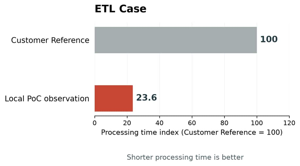
Figure 2. ETL Case. Recorded duration indexed to Customer Reference = 100. The local result averages two measured cycles; input volumes differed. This observation does not establish equivalent-workload platform performance.
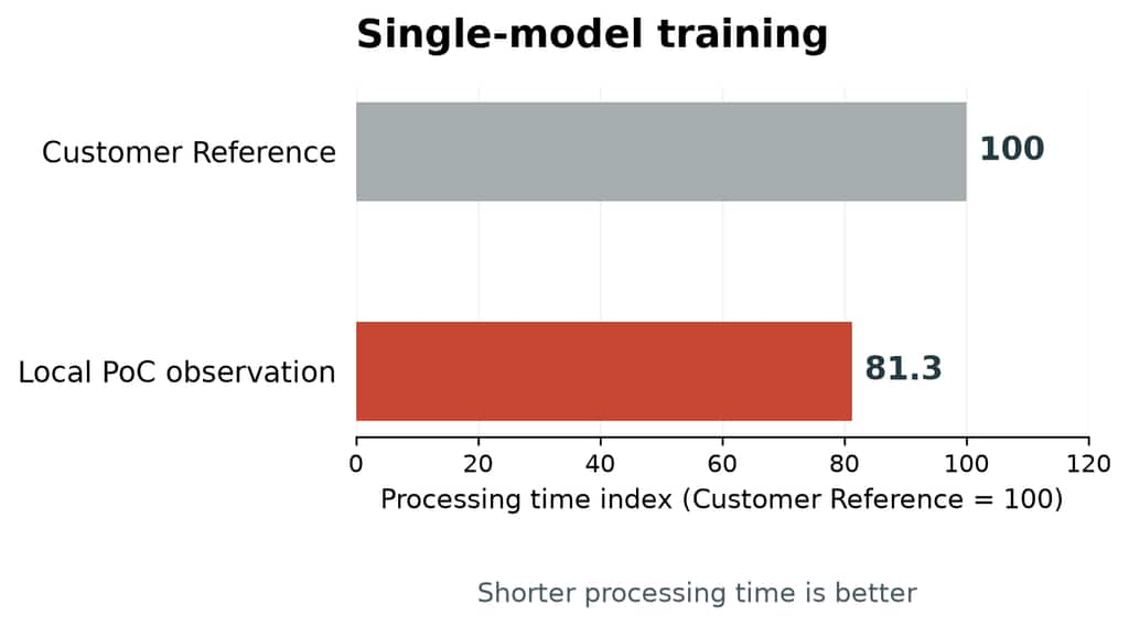
Figure 3. Single-model training. Recorded single-model training duration indexed to Customer Reference = 100. This case covers training, rather than the complete MLOps workflow. Validation error was higher in the local test; shorter duration does not establish equivalent-quality training performance.
The ETL result averages two local processing cycles using memory-backed working storage. Input volumes differed from the customer reference, so the chart shows the recorded case timings rather than a platform speedup for the same workload.
The single-model training case used a controlled historical test dataset. Validation error was higher in the local test; shorter duration does not establish equivalent-quality training performance. These observations do not establish production forecast quality.
The observations cover local processing. They exclude publication, ADB loading, and query serving, and do not measure end-to-end application latency. For a low-latency use case, we would also test the full path from data generation to the application’s response.
From local processing to business value
With this approach, you can bring an existing pipeline to the customer site for a residency requirement, a latency requirement, or both. ADB adds a way to support scheduled runs and connect policy-selected outputs to the people and applications that use them.
In telecommunications, forecasts and anomaly results could help teams prepare capacity for changing demand, plan for holidays or large events, and identify low-demand periods for energy optimization. Dashboards provide a way to examine these outputs and decide where to act. AI-assisted access could be added after its data handling and behavior are validated.
Faster processing can make results available sooner. How useful they are will also depend on the data, model quality, and integration with operational systems. For the operations team, the value comes when the information arrives in time to help with a decision.
Conclusion
This architecture connects local ETL and MLOps execution to Oracle Autonomous AI Database for scheduling support and access to published results. You can use the pattern when raw data needs to stay within a defined boundary, when processing needs to be close to data generation, or when both apply. The configuration and publication policy determine how that boundary is maintained.
Our approach retained most of the existing pipeline code and logic, with limited migration changes. Two levels of optimization focused on adapting execution and tuning for the local infrastructure. The deployment still needs testing against its own data policy, processing workload, output-quality goals, and application response time.
Three takeaways:
- Bring processing to the data: local execution can help with data residency requirements, low-latency applications, or both.
- Make the integration explicit: combine Oracle Scheduler with solution-owned execution, run tracking, and publication components, and define what each cloud path may carry.
- Optimize around the pipeline: retain existing code where practical, make the migration changes needed, and evaluate execution configuration and infrastructure tuning with representative workloads.
Acknowledgments
This project was a joint effort among the JAPAC Cloud Engineering, JAPAC Center of Excellence (CoE), and JAPAC Sales teams. We thank Joey Boo, Kiat Hong Tay, and Mun Yoke Wong for their help and contributions. We also thank Joshua Bendicion Chua, together with the wider Oracle product and engineering teams, for their guidance and support. The architecture, solution development, and validation described here reflect this collaboration.
References
1. Oracle Roving Edge Infrastructure.
2. Oracle Compute Cloud@Customer frequently asked questions.
3. Creating and managing jobs with Oracle Scheduler.