Introduction to Vector Similarity Search

What is Vector Similarity Search? With regular search we usually rely on exact matches. The item either exists or it does not. With Vector Similarity Search, or VSS, we search for items that are semantically similar. Instead of comparing strings directly, we compare embeddings. Embeddings are numeric vectors that represent the meaning of text, images, documents, or other data. For example, these two questions are different strings:

“What is semantic caching?”
“Can you explain semantic caching?”

A traditional search may treat them as completely different requests. But vector similarity search can recognize that they are asking for almost the same thing.

What Are Vectors?

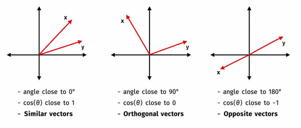
A vector is a sequence of numbers with magnitude and direction. In simple diagram below, we can show vectors in two dimensions. If two vectors point in roughly the same direction, they are similar. If they are close to 90 degrees apart, they are orthogonal and generally unrelated. If they point in opposite directions, they are very dissimilar.

In real-world embedding systems, vectors are not two-dimensional. They usually have hundreds or thousands of dimensions.

[-0.046452742, -0.004415608, 0.013397201, 0.026726048, 0.001498641, -0.027806027, -0.028735628, 0.037402797, 0.013738966, -0.0077238963, 0.0130349295, ...]

[-0.027806787, 0.00070229557, 0.0041609216,-0.019758206, 0.016464725, -0.027134277, 0.01724345, 0.010519548, 0.011608103, -0.004154951, -0.004082942, …]

These numbers are not meant to be interpreted individually. What matters is how the entire vector compares to other vectors. There are several approaches we can take for comparing vectors.

Cosine Similarity

Cosine similarity is a very common approach for vector simillarity search. It compares the angle between two vectors. It does not care about the magnitude, or size, of the vectors. It only cares whether they point in a similar direction. The result is usually interpreted like this:

Close to 1: very similar
Close to 0: unrelated or orthogonal
Close to -1: opposite direction

L2 / Euclidean Distance

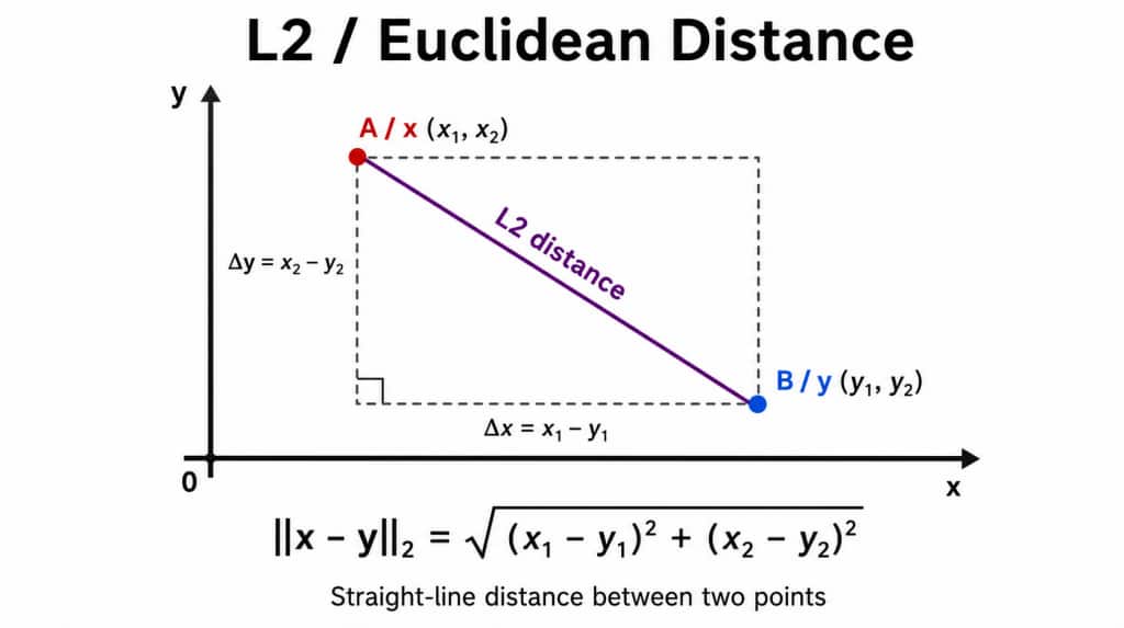
Euclidean distance, also called L2 distance, measures the straight-line distance between two vectors in multi-dimensional space. A smaller distance means the vectors are more similar. This is based on the Pythagorean theorem. In practice, systems may avoid calculating the square root and compare squared distances instead, because it is cheaper computationally and preserves the same ordering. Euclidean distance cares about actual coordinate distance, not just direction.

Inner product

Inner product, also called dot product, multiplies corresponding vector components and sums the results.

A = [1, 2]
B = [3, 4]
C = [-5, -6]

The inner product of A and B is:

A.B = 1*3 + 2*4 = 11

The inner product of A and C is:

A.C = 1*-5 + 2*-6 = -17

This tells us that A and B point more in the same direction than A and C.

In general:

Same direction: large positive value
Unrelated: near zero
Opposite direction: negative value

Normalized (unit) vector

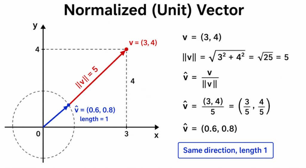
This is another important topic to consider. For example, take this vector: [3, 4]

Its magnitude is: sqrt(3² + 4²) = 5

To normalize it, we divide each component by 5: [3/5, 4/5] = [0.6, 0.8]

The direction stays the same, but the magnitude becomes 1.

This matters because when vectors are normalized, inner product becomes equivalent to cosine similarity.

For example: A = [1, 0] B = [0.707, 0.707]

The angle between these vectors is approximately 45 degrees.

The inner product is: 1*0.707 + 0*0.707 = 0.707

And: cos(45°) = 0.707

So for normalized vectors, inner product and cosine similarity produce the same similarity score.

How Do We Compare Many Vectors?

Comparing two vectors is simple. Comparing millions or billions of vectors is much harder. A brute-force search compares the query vector against every stored vector. This is accurate, but it has O(N) complexity, which becomes expensive as the dataset grows. To solve this, many vector databases use Approximate Nearest Neighbor, or ANN, algorithms. One popular ANN algorithm is HNSW, which stands for Hierarchical Navigable Small World.

HNSW: Hierarchical Navigable Small World

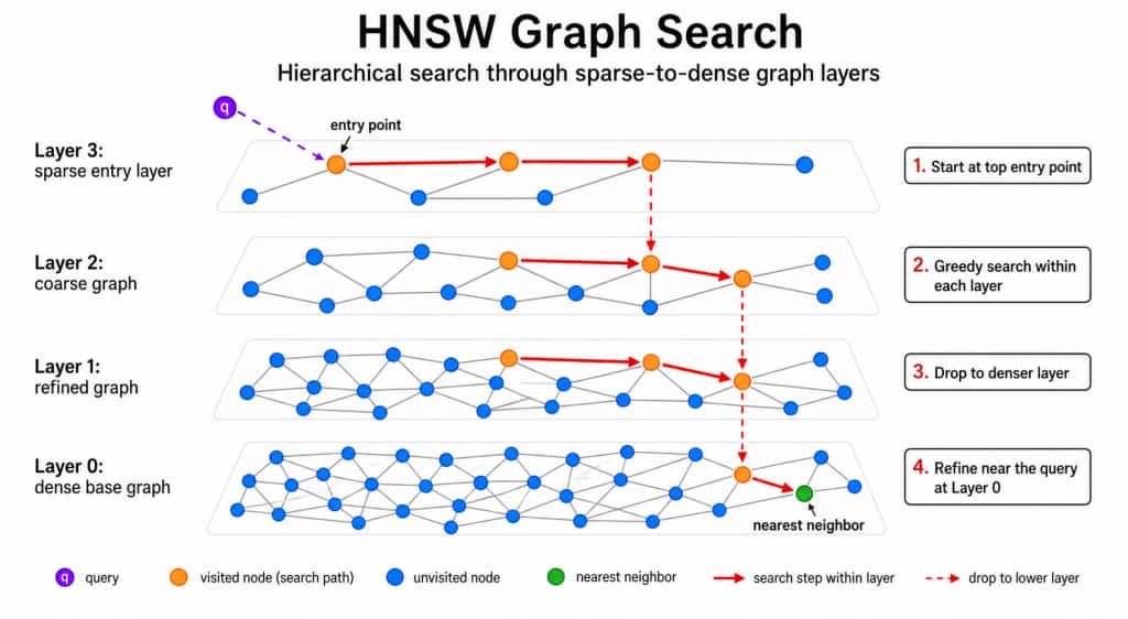
HNSW allows fast similarity search across large vector datasets. Instead of comparing the query against every vector, it builds a graph structure that helps navigate quickly toward the closest matches.

The HNSW index contains multiple layers.

The top layer has sparse connections and only a small number of vectors. You can think of it like highways for fast global navigation.
The middle layers have more vectors and denser connections. They are like major roads that help refine the search.
The bottom layer contains all vectors. This is where the most precise local search happens, and it is also where most of the memory is used.

As the number of vectors grows, more layers are usually needed:

10K vectors -> approximately 4-5 layers
1M vectors -> approximately 6-8 layers
100M vectors -> approximately 9-12 layers

HNSW search generally works like this:

Start at a random node in the top layer.
Compare that node to the query vector.
Move to the neighboring node closest to the query.
Drop down to the next layer.
Repeat the process until reaching the bottom layer.
Return the closest candidates.

The main benefits of HNSW are speed and high recall. The main downside is memory usage.

HNSW Memory Usage

HNSW stores both vectors and graph connections. Vector memory depends on the number of dimensions and the data type. For float32, each dimension uses 4 bytes. For example: 4096 dimensions * 4 bytes = 16,384 bytes. Graph connections also require memory. If each node has M = 16 neighbors and each pointer uses 8 bytes: 16 neighbors * 8 bytes = 128 bytes. There is also additional overhead for metadata and indexing structures. This is why HNSW is fast, but memory-intensive.

Alternatives to HNSW

HNSW is not the only approach. For small datasets, a flat or brute-force index may be acceptable. It is simple and accurate, but slow at large scale. For very large datasets, such as billions of vectors, other approaches may be use. The right choice depends on dataset size, accuracy requirements, latency requirements, and memory budget but here are possible choices.

Inverted File Index

Inverted File Index, or IVF, is a method used to speed up vector similarity search. Instead of comparing a query vector against every vector in a database, IVF first groups vectors into clusters. Each cluster has a representative center, often called a centroid. When a query comes in, the system finds the closest centroids, then searches only inside those nearby clusters.

For example, if a database has 1 million vectors, IVF might divide them into 1,000 clusters. A query may search only the 5 or 10 closest clusters instead of all 1 million vectors. This makes search much faster. The tradeoff is accuracy. If the best match is in a cluster that was not searched, the system may miss it. To improve accuracy, IVF can search more clusters, but that also takes more time.

In short, IVF speeds up vector search by narrowing the search area to the most promising groups of vectors.

Product Quantization

Product Quantization, or PQ, is a compression method used in vector similarity search. It works by splitting a large vector into smaller parts, then replacing each part with a nearby representative value from a small codebook. Instead of storing the full vector, the system stores short codes that approximate it.

This greatly reduces memory usage and makes similarity search faster, especially for very large datasets. For example, a high-dimensional vector that normally takes a lot of storage can be represented with a much smaller compressed code. The tradeoff is precision. Because PQ stores an approximation, search results may be slightly less accurate than using the original full vectors.

In short, Product Quantization makes vector search cheaper and faster by compressing vectors, while accepting a small loss in accuracy.

Conclusion

To summarize Vector Similarity Search is a technique for finding information based on meaning or similarity rather than exact keyword matches. It works by converting data such as text, images, or audio into numerical vectors called embeddings. Items with similar meaning are placed close together in vector space, allowing a system to quickly find the most relevant matches to a query.

Vector Similarity Search has numerous benefits. It searches by meaning instead of exact words, handles synonyms and related ideas well, and is useful for search and recommendations. However, it depends on high-quality embeddings, can sometimes return irrelevant results, is harder to explain than keyword search, and requires extra storage and tuning.

In a future post, I will explore how Vector Similarity Search enables Semantic Caching.

Introduction to Vector Similarity Search