In this article, we explore how fundamental geometric shapes – points, lines, and polygons – enable spatial analysis and mapping. Geospatial data comes in many forms, such as raw coordinates in CSVs and databases, GeoJSON, or shapefiles. To visualize and analyze these spatial elements together, they must be converted into a common format: the geometry data type. Once converted, Oracle Analytics can map them as layers on the same map and run spatial operations.
Three Core Geometry Types
Points
A point represents a single location on Earth defined by a coordinate pair (latitude and longitude).
- Examples: Customer address, mobile tower, drop-off location
- Geometry Format: POINT(78.4867 17.3850)
Lines
A line, also called a line string, connects two or more points to represent movement, direction, or connectivity.
- Examples: Shipping route, fiber cable, or storm path
- Geometry Format: LINESTRING(78.48 17.38, 80.27 13.08)
Polygons
A polygon is a closed shape that defines areas or boundaries.
- Examples: City limits, flood zones, or sales territories
- Geometry Format: POLYGON((78.4 17.3, 78.6 17.3, 78.6 17.5, 78.4 17.5, 78.4 17.3))
These geometry types can be stored in Oracle databases using SDO_GEOMETRY or directly in CSV datasets using the Well-Known Text (WKT) format. Oracle Analytics natively supports both methods for map rendering and analysis.
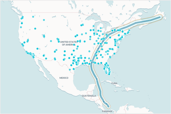
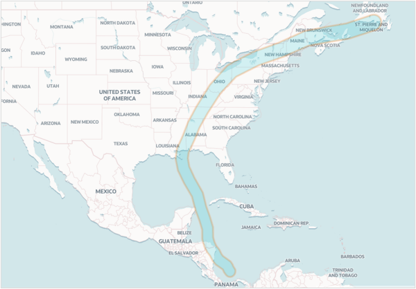
Example Use Case: Identifying Customers Affected by a Storm
Suppose you work for a utility company and need to determine which customer locations may be impacted by a storm. You would use:
- Points for customer locations
- A line for the storm path
- A polygon to create a buffer zone around the storm path
Oracle Analytics allows these layers to be visualized together on a single map.
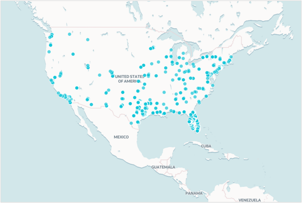
Step 1: Convert Locations to Points
If your data is stored in an Oracle database, you can convert latitude and longitude values into point geometry using SQL. For data in spreadsheets, several GIS tools including desktop applications and online converters can help transform coordinates into CSV files with WKT format. Once uploaded, Oracle Analytics detects the geometry column and visualizes it automatically.
For more details on working with data stored in an Oracle database, see Learn how to spatially enable a table, register metadata, and create spatial indexes.
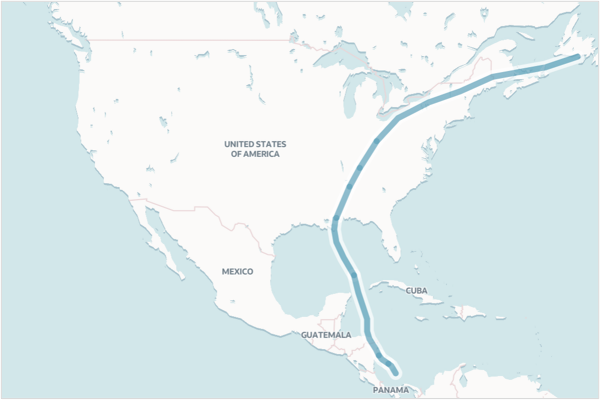
Step 2: Import Line and Polygon Data
If the storm path is provided in a GeoJSON or shapefile, you can upload it to an Oracle Autonomous Database using tools like Data Studio or Oracle Spatial Studio, which store the geometry in the appropriate format. Alternatively, desktop GIS applications or online tools can export the geometry as WKT in a CSV file. These tools can also help clean up GeoJSON files by removing unsupported M (measure) and Z (elevation) dimensions.
For more details on loading spatial data into an Oracle database, refer to the documentation on uploading common geospatial formats using Oracle tools such as Spatial Studio or Data Studio, see Loading GeoJSON – Oracle ADB Documentation and Uploading a Shapefile in Spatial Studio.
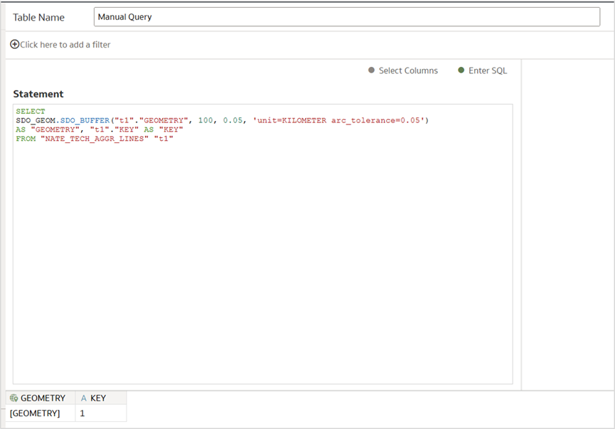
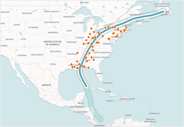
Step 3: Create a Buffer Zone
To model a risk zone, you can create a buffer around the storm path using the SDO_GEOM.SDO_BUFFER function in Oracle Database. For example, a 100-kilometer buffer polygon can highlight at-risk areas. You can create this buffer with a manual Spatial SQL and save it as a dataset within Oracle Analytics, then visualized as a map layer.
Spatial SQL: Create a 100 km buffer around a storm path
SELECT

  SDO_GEOM.SDO_BUFFER(

    t1.GEOMETRY,

    100,

    0.05,

    'unit=KILOMETER arc_tolerance=0.05'

  ) AS GEOMETRY,

  t1.KEY AS KEY

FROM NATE_TECH_AGGR_LINES t1;
For more details, see SDO_BUFFER.
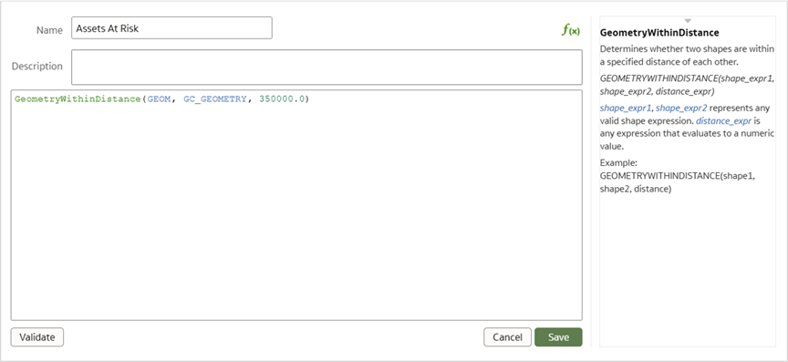
Step 4: Perform Spatial Analysis Without Code
Oracle Analytics includes built-in functions like GeometryWithinDistance that help identify spatial relationships. For instance, to find customer assets within 350 kilometers of a storm path, use the expression GEOMETRYWITHINDISTANCE(“stormpath”, “customerassets”, 350000).
This returns a true or false value, which can be used to filter, highlight, or analyze affected customers.
Stay Tuned
In the next part of this series, we’ll explore Spatial SQL to dynamically change the buffer risk zone using session variables and parameter binding.
Reference
Geometry Data Type technical paper
Call to Action
Now that you’ve read this article, try it yourself and let us know your results in the Oracle Analytics Community, where you can also ask questions and post ideas. Be sure to explore the Community Gallery as well, where users share their most creative dashboards and map visualizations for inspiration.