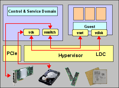
 Finally finding some time to continue this blog series… And starting the new year with a new chapter for which I hope to write several sections: Physical IO options for LDoms and what you can do with them. In all previous sections, we talked about virtual IO and how to deal with it. The diagram at the right shows the general architecture of such virtual IO configurations. However, there’s much more to IO than that.
From an architectural point of view, the primary task of the SPARC hypervisor is partitioning of the system. The hypervisor isn’t usually very active – all it does is assign ownership of some parts of the hardware (CPU, memory, IO resources) to a domain, build a virtual machine from these components and finally start OpenBoot in that virtual machine. After that, the hypervisor essentially steps aside. Only if the IO components are virtual components, do we need hypervisor support. But those IO components could also be physical. Actually, that is the more “natural” option, if you like. So lets revisit the creation of a domain:
We always start with assigning of CPU and memory in some very simple steps:
root@sun:~# ldm create mars
root@sun:~# ldm set-memory 8g mars
root@sun:~# ldm set-core 8 mars
If we now bound and started the domain, we would have OpenBoot running and we could connect using the virtual console. Of course, since this domain doesn’t have any IO devices, we couldn’t yet do anything particularily useful with it. Since we want to add physical IO devices, where are they?
To begin with, all physical components are owned by the primary domain. This is the same for IO devices, just like it is for CPU and memory. So just like we need to remove some CPU and memory from the primary domain in order to assign these to other domains, we will have to remove some IO from the primary if we want to assign it to another domain. A general inventory of available IO resources can be obtained with the “ldm ls-io” command:
root@sun:~# ldm ls-io
NAME                                      TYPE   BUS      DOMAIN   STATUS
----                                      ----   ---      ------   ------
pci_0                                     BUS    pci_0    primary
pci_1                                     BUS    pci_1    primary
pci_2                                     BUS    pci_2    primary
pci_3                                     BUS    pci_3    primary
/SYS/MB/PCIE1                             PCIE   pci_0    primary  EMP
/SYS/MB/SASHBA0                           PCIE   pci_0    primary  OCC
/SYS/MB/NET0                              PCIE   pci_0    primary  OCC
/SYS/MB/PCIE5                             PCIE   pci_1    primary  EMP
/SYS/MB/PCIE6                             PCIE   pci_1    primary  EMP
/SYS/MB/PCIE7                             PCIE   pci_1    primary  EMP
/SYS/MB/PCIE2                             PCIE   pci_2    primary  EMP
/SYS/MB/PCIE3                             PCIE   pci_2    primary  OCC
/SYS/MB/PCIE4                             PCIE   pci_2    primary  EMP
/SYS/MB/PCIE8                             PCIE   pci_3    primary  EMP
/SYS/MB/SASHBA1                           PCIE   pci_3    primary  OCC
/SYS/MB/NET2                              PCIE   pci_3    primary  OCC
/SYS/MB/NET0/IOVNET.PF0                   PF     pci_0    primary
/SYS/MB/NET0/IOVNET.PF1                   PF     pci_0    primary
/SYS/MB/NET2/IOVNET.PF0                   PF     pci_3    primary
/SYS/MB/NET2/IOVNET.PF1                   PF     pci_3    primary
The output of this command will of course vary greatly, depending on the type of system you have. The above example is from a T5-2. As you can see, there are several types of IO resources. Specifically, there are
- BUS
This is a whole PCI bus, which means everything controlled by a single PCI control unit, also called a PCI root complex. It typically contains several PCI slots and possibly some end point devices like SAS or network controllers. - PCIE
This is either a single PCIe slot. In that case, it’s name corresponds to the slot number you will find imprinted on the system chassis. It is controlled by a root complex listed in the “BUS” column. In the above example, you can see that some slots are empty, while others are occupied. Or it is an endpoint device like a SAS HBA or network controller. An example would be “/SYS/MB/SASHBA0” or “/SYS/MB/NET2”. Both of these typically control more than one actual device, so for example, SASHBA0 would control 4 internal disks and NET2 would control 2 internal network ports. - PF
This is a SR-IOV Physical Function – usually an endpoint device like a network port which is capable of PCI virtualization. We will cover SR-IOV in a later section of this blog.
All of these devices are available for assignment. Right now, they are all owned by the primary domain. We will now release some of them from the primary domain and assign them to a different domain. Unfortunately, this is not a dynamic operation, so we will have to reboot the control domain (more precisely, the affected domains) once to complete this.
root@sun:~# ldm start-reconf primary
root@sun:~# ldm rm-io pci_3 primary
root@sun:~# reboot
[ wait for the system to come back up ]
root@sun:~# ldm add-io pci_3 mars
root@sun:~# ldm bind mars
With the removal of pci_3, we also removed PCIE8, SYSBHA1 and NET1 from the primary domain and added all three to mars. Mars will now have direct, exclusive access to all the disks controlled by SASHBA1, all the network ports on NET1 and whatever we chose to install in PCIe slot 8. Since in this particular example, mars has access to internal disk and network, it can boot and communicate using these internal devices. It does not depend on the primary domain for any of this. Once started, we could actually shut down the primary domain. (Note that the primary is usually the home of vntsd, the console service. While we don’t need this for running or rebooting mars, we do need it in case mars falls back to OBP or single-user.)
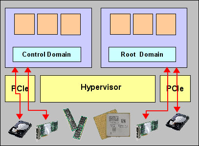 Mars now owns its own PCIe root complex. Because of this, we call mars a root domain. The diagram on the right shows the general architecture. Compare this to the diagram above! Root domains are truely independent partitions of a SPARC system, very similar in functionality to Dynamic System Domains in the E10k, E25k or M9000 times (or Physical Domains, as they’re now called). They own their own CPU, memory and physical IO. They can be booted, run and rebooted independently of any other domain. Any failure in another domain does not affect them. Of course, we have plenty of shared components: A root domain might share a mainboard, a part of a CPU (mars, for example, only has 2 cores…), some memory modules, etc. with other domains. Any failure in a shared component will of course affect all the domains sharing that component, which is different in Physical Domains because there are significantly fewer shared components. But beyond this, root domains have a level of isolation very similar to that of Physical Domains.
Comparing root domains (which are the most general form of physical IO in LDoms) with virtual IO, here are some pros and cons:
Pros:
- Root domains are fully independet of all other domains (with the exception of console access, but this is a minor limitation).
- Root domains have zero overhead in IO – they have no virtualization overhead whatsoever.
- Root domains, because they don’t use virtual IO, are not limited to disk and network, but can also attach to tape, tape libraries or any other, generic IO device supported in their PCIe slots.
Cons:
- Root domains are limited in number. You can only create as many root domains as you have PCIe root complexes available. In current T5 and M5/6 systems, that’s two per CPU socket.
- Root domains can not live migrate. Because they own real IO hardware (with all these nasty little buffers, registers and FIFOs), they can not be live migrated to another chassis.
Because of these different characteristics, root domains are typically used for applications that tend to be more static, have higher IO requirements and/or larger CPU and memory footprints. Domains with virtual IO, on the other hand, are typically used for the mass of smaller applications with lower IO requirements. Note that “higher” and “lower” are relative terms – LDoms virtual IO is quite powerful.
This is the end of the first part of the physical IO section, I’ll cover some additional options next time. Here are some links for further reading:
- Admin Guide: Creating Root Domains
- Whitepaper: “Implementing Root Domains with OVM Server for SPARC” (pdf)
- Root Complex Layout in