In this blog entry, we will describe how to use reinforcement learning techniques in the context of BPF programs. Specifically we will talk about how reinforcement learning can help solve BPF-driven auto-tuning challenges for bpftune in the context of choosing a TCP congestion control algorithm appropriate for current network conditions.
In a previous blog post, we talked about bpftune, which provides BPF-based tuners to auto-tune aspects of Linux. bpftune is an open-source project, and while we started the ball rolling with tuning issues experienced here at Oracle, our hope is it can grow to handle many more tuning scenarios. In fact bpftune was designed to be modular to allow easy extensibility to cover additional subsystems; such tuners can be delivered as part of core bpftune or separately. The feature plan is maintained in the github repo describing what problems have been solved so far, and what ideas we have for future work.
I talked about bpftune at the eBPF summit 2023. The video from that talk is here.
I also spoke recently about bpftune, BPF and reinforcement learning on Liz Rice’s excellent eCHO eBPF podcast – it is a great resource for learning about BPF.
Introduction
We recently replaced an explicit algorithm – “use BBR for TCP connections to remote hosts that have experienced packet loss” – with reinforcement learning methods. The advantanges of using reinforcement learning are:
- Reinforcement learning is an online learning method; it learns all the time and does not require pre-training.
- Reinforcement learning is easily implemented in BPF. BPF – while powerful – is a restricted environment for safety reasons. So being able to implement a learning method with no floating point division for example is a win.
- Reinforcement learning converges quickly; i.e. it learns fast.
- The reinforcement algorithm used adapts to a wider range of scenarios; the fixed approach used previously only handled loss situations.
Before we describe the specifics of the algorithm used, we will briefly discuss what reinforcement learning is; then we will see how it can be applied to the problem of choosing a TCP congestion control algorithm.
A Quick Introduction to Reinforcement Learning
Reinforcement learning is an action-oriented learning approach where an agent takes actions in an environment, and based upon reward signals from the environment attempts to maximize those rewards over time.
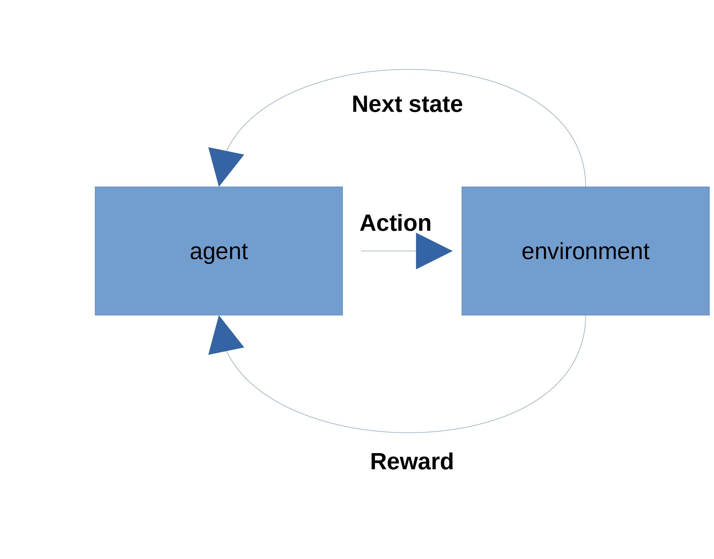
An agent takes a set of actions in an environment, transitioning to different states, and may or may not receive rewards along the way. Some reinforcement learning tasks break naturally into episodes (like a game of chess). In such cases, we attempt to learn the overall reward – termed the gain – for a given state across all episodes, and over time we both use that estimate to guide behaviour and refine the estimate as we observe the consequences of our actions. This sort of bootstrapping is the key to reinforcement learning; we “learn on the job”.
This form of learning dovetails neatly with bpftune, whose guiding philosophy is to make small changes in behaviour to see if they benefit the system while watching out for negative side-effects.
A key assumption underlying reinforcement learning is that states have the Markov property – that when in a given state, history prior to reaching that state is irrelevant. So any time we enter a state we can use past experience of that state to guide behaviour, without having to worry how we got to the state. This allows us to associate values with states meaningfully.
An agent learns a value function – a means of associating expected rewards with states and actions. A key question is how to act – do we maximize reward all the time, always picking the state/action that leads to the highest reward (exploitation)? Or do we sometimes explore the environment also to see if other states might yield better rewards in the future?
The behavioural choices an agent makes are termed its policy. A key question for policy formulation is whether the environment is static or non-stationary – in the latter case exploration will always be needed as old evaluations of actions or states may no longer be valid.
TCP Congestion Control – A Quick Primer
TCP uses a sliding window with TCP sequence numbers, and the size of the window is negotiated between the two sides of the TCP connection. However, once we move to a world with a lot of different TCP connections (and other forms of network traffic), we have to consider other aspects apart from the two ends of the connection. When setting out on a car journey, we need to consider both the likliehood that there will be a parking space at the destination (the TCP window is open) and if we will hit any traffic jams along the way (congestion). Ignoring the possibility of congestion – where a network has more traffic than it can handle – is a problem, because protocols like TCP will retransmit in the face of loss, and this can increase congestion in some cases. So protocols like TCP have to find ways to observe and react to congestion so that they avoid congestion collapse – where the congestion prevents or limits useful communication.
Congestion control algorithms have typically used packet loss as a signal of congestion, but some newer alogrithms such as BBR try to model the behaviour of the communication pathway instead, as the traditional approach could sometimes under-estimate traffic capacity.
How bpftune Picks a Congestion Control Algorithm
In applying reinforcement learning to TCP congestion control algorithm choice, we take the approach that
- a TCP connection lifetime is an “episode” in reinforcement learning terms.
- at connection initiation (either accept or connect), we take an action to select a congestion control algorithm.
- at episode end (connection close) we use information about the connection to comprise a reward signal associated with the congestion algorithm chosen.
- because the environment is non-stationary (network conditions can change), a purely greedy approach where we select the algorithm to maximize reward will not work. An epsilon-greedy approach – where we select the greedy action most of the time, but with a small probability (epsilon) select a non-greedy action to explore the environment – should be used.
- we make TCP congestion control algorithm choice on a per-remote host basis; other ways of making the choice are possible of course, such as per-service, but since this approach is about learning datapath characteristics, a per-remote host approach makes most sense.
How to make all of this work in BPF? We have some constraints:
- we need to have a way to catch connection setup and close and be able to set congestion control algorithm at connection setup time. Happily BPF provides “sockops” BPF programs that can be triggered at connection connect() or accept() time, and then can be configured to trigger on TCP state changes. The latter allows us to observe the closing state. The helper bpf_setsockopt() can be used to set congestion control algorithm at connection setup time.
- our algorithm selection needs to happen within a running BPF program, so we need to do things like espilon-greedy choice in BPF context. The good news is we have pseudo-random number generation in the form of BPF helper bpf_get_prandom_u32(), so we can use it to select random states.
- we can only use integer division, so any metrics need to take that into account.
In specific terms of metric choice, the BBR paper notes that the optimal operating point for a congestion algorithm to work is at the bandwidth delay product (BDP), which comprises the product of the actual round-trip propagation time of the link and the bottleneck bandwidth – the bandwidth of the choke point along the channel of communication. If we operate at or near this point, we are filling the communication pipe as much as possible without overfilling it (which leads to congestion).
A good estimate of the round-trip propagation time is the minimum TCP round-trip-time (RTT) that we see, while a good estimate of the bottleneck bandwidth is the maximum packet delivery rate we observe. BBR uses these estimates, but we can use them also to compare across congestion control algorithms.
So our metric for congestion control algorithms boils down to this; a good algorithm choice should approach the minimum RTT observed and the maximum packet delivery rate. On an intuitive level, it is a metric that covers both latency (min RTT) and throughput (packet delivery rate).
We will now walk through the various aspects of the implementation in a bit more detail.
What BPF program type is suitable?
For TCP sockets, we use a TCP-BPF “sockops” BPF program. The BPF program is attached to the root cgroup – this means it will fire for all connection established and connection accepted events for all TCP sockets on the system. From there, we enable additional TCP state change events, such that the program will also run when a TCP connection in the given cgroup changes state. When we encounter a state change event, we only want TCP state changes that indicate the connection is closing; this is where we will update our metrics based upon the connection performance. See here for the BPF code used by the TCP connection tuner.
SEC("sockops")
int conn_tuner_sockops(struct bpf_sock_ops *ops)
{
    int cb_flags = BPF_SOCK_OPS_STATE_CB_FLAG;
    struct bpf_sock *sk = ops->sk;
...

    switch (ops->op) {
    case BPF_SOCK_OPS_ACTIVE_ESTABLISHED_CB:
    case BPF_SOCK_OPS_PASSIVE_ESTABLISHED_CB:
        /* enable other needed events */
        bpf_sock_ops_cb_flags_set(ops, cb_flags);
        ...
        break;
    case BPF_SOCK_OPS_STATE_CB:
    state = ops->args[1];
    switch (state) {
    case BPF_TCP_FIN_WAIT1:
        case BPF_TCP_CLOSE_WAIT:
            if (!sk)
                return 1;
            break;
        default:
            return 1;
        }
Metric storage
We use multiple sets of metrics – one for each congestion control algorithm. These are stored in a BPF hash map keyed by remote IP address; as noted above, we are trying to find the congestion control algorithm that is best for the data path, so per-remote host metrics make sense. See here for the data structure definitions.
For each congestion control algorithm, we store metrics as follows:
struct tcp_conn_metric {
        __u64 state_flags;  /* state/action - cong alg used */
        __u64 greedy_count;     /* amount of times greedy option was taken */
        __u64 min_rtt;      /* min RTT observed for this cong alg */
        __u64 max_rate_delivered; /* max rate delivered for this cong alg */
        __u64 metric_count; /* how many metrics collected? */
        __u64 metric_value;
};
We store an array of these – one for each congestion control algorithm – in a “struct remote host”; it is looked up via the remote IP address associated with the TCP connection, available in the “struct sock_ops”:
struct remote_host {
        __u64 min_rtt;
        __u64 max_rate_delivered;
        struct tcp_conn_metric metrics[NUM_TCP_CONN_METRICS];
};
We use that structure to keep track of the overall minimum RTT observed across all connections/congestion control algorithms and the maximum rate of packet delivery.
Normally in reinforcement learning, we need to distinguish between states and actions; i.e. in state X take action A to reach state Y. In our case, we can make states synonymous with actions; from an initial state, choose a congestion control algorithm A to enter state A. Because we only have one action choice for a connection at this time – choose a congestion control algorithm – we simply attribute any metrics to the state associated with that action. So in the following discussion, states/actions may be used interchangeably to refer to the congestion algorithm choice. It is to that choice we ascribe our metric values. In a more complicated model, a sharper distinction would likely need to be drawn.
Choosing an action
Here we show how to choose among the TCP metrics associated with different congestion control algorithms. The metric – and associated congestion control algorithm – which has the minimum value is chosen. The complication is we can have multiple candidates with equal values; in that case we pick randomly among them.
    __u64 metric_value = 0, metric_min = ~((__u64)0x0);
    __u8 i, ncands = 0, minindex = 0, s;
    __u8 cands[NUM_TCP_CONN_METRICS];

    /* find best (minimum) metric and use cong alg based on it. */
    for (i = 0; i < NUM_TCP_CONN_METRICS; i++) {
        metric_value = remote_host->metrics[i].metric_value;
        if (metric_value > metric_min)
             continue;
        if (metric_value < metric_min) {
            cands[0] = i;
            ncands = 1;
        } else if (metric_value == metric_min) {
            cands[ncands++] = i;
        }
        metric_min = metric_value;
    }
So we pick out one or more candidate states that have mimimum metric value. If we have more than one candidate, we simply choose randomly between them:
    /* if multiple min values, choose randomly. */
    if (ncands > 1) {
        int choice = bpf_get_prandom_u32() % ncands;

        /* verifier refused to believe the index used was valid, so
         * unroll the mapping from choice to cands[] index to keep
         * verification happy.
         */
        switch (choice) {
        case 0:
            minindex = cands[0];
            break;
        case 1:
            minindex = cands[1];
            break;
        case 2:
            minindex = cands[2];
            break;
        case 3:
            minindex = cands[3];
            break;
        default:
            return 1;
        }
    } else if (ncands == 1) {
        minindex = cands[0];
    } else {
        return 1;
    }
Epsilon-greedy action/state choice
We use an epsilon-greedy strategy, where we mostly pick the optimal greedy action (chosen above), but sometimes pick a random action among the num_states with a specific probability. Here the probability is expressed in how often we pick a suboptimal state; epsilon == 20 means one in 20 times the state is chosen randomly. Remember we have no floating-point support, so we cannot deal in probabilities like 0.05!
/* choose random state every epsilon states */
static __always_inline int epsilon_greedy(__u32 greedy_state, __u32 num_states,
                                          __u32 epsilon)
{
    __u32 r = bpf_get_prandom_u32();

    if (r % epsilon)
        return greedy_state;
    /* need a fresh random number, since we already know r % epsilon == 0. */
    r = bpf_get_prandom_u32();
    return r % num_states;
}
Metric (reward) calcuation
For a TCP connection, we need to calcuate the associated metric and update the reward value (in this case a higher value means a lower reward) associated with the congestion algorithm that was used for that connection.
First we compute the metric; we want to reward (with lower values) connections that had low minimum RTTs relative to the mimimum RTT observed for the remote system, and high packet delivery rates relative to the maximum observed for the remote system.
The metric is computed as follows:
static __always_inline __u64 tcp_metric_calc(struct remote_host *r,
                                             __u64 min_rtt,
                                             __u64 rate_delivered)
{
    __u64 metric = 0;

    if (!r->min_rtt || min_rtt < r->min_rtt)
        r->min_rtt = min_rtt;
    if (!r->max_rate_delivered || rate_delivered > r->max_rate_delivered)
        r->max_rate_delivered = rate_delivered;
    if (r->min_rtt)
        metric += ((min_rtt - r->min_rtt)*RTT_SCALE)/r->min_rtt;
    if (r->max_rate_delivered)
        metric +=
            ((r->max_rate_delivered - rate_delivered)*DELIVERY_SCALE)/
            r->max_rate_delivered;
    return metric;
}
In the first computation, we use the difference between the minimum RTT observed for the specific connection and the overall minimum RTT observed; it is then multiplied by a scaling factor (to faciliate integer division) and divided by the overall min RTT rate; so we essentially get something like the percentage above the overall min RTT value. A similar approach is taken for the delivery rate. So a connection with RTT approaching the minimum, and high packet delivery rate will be favoured with a lower metric value.
In testing this approach, we discovered that while we can use the current connection minimum RTT to compute the metric, the delivery rate for each connection varies too much. Different traffic characteristics of different services get lumped together, and while the RTT is stable acrosss different service types for the most part, packet delivery rates can vary. As a result, when computing our metric, we use the minimum RTT for the specific connection and the maximum delivery rate observed for the given congestion control algorithm, not the specific connection. This performs better in practice and is a more stable basis for metric computation.
Finally we need to update the overall value for the congestion control algorithm chosen using the latest metric we have obtained. The approach taken is to use something like the delta rule in neural networks; we want our updated value to more closely resemble the value we just got, but also reflect its historic value since it is possible the current value was not typical. So we update the value with a fraction of the difference between the current value and the metric – the fraction is the learning rate. Instead of using a learning rate like 0.1, we use bitshifts where each shift to the right halves the difference:
static __always_inline __u64 rl_update(__u64 value, __u64 metric, __u8 bitshift)
{
    if (!value)
        return metric;
    if (metric > value)
        return value + ((metric - value) >> bitshift);
    else if (metric < value)
        return value - ((value - metric) >> bitshift);
    else
        return value;
}
bpftune defaults to a learning rate of 0.25 (two bit shifts right), which seems high, but helps fast convergence.
So over time, the value we associate with a congestion control algorithm becomes better attuned to the metrics we observe.
Benchmarking bpftune TCP performance
So how does this all work in practice?
Here we evaluate the choices made by bpftune under various loss and latency conditions.
First, let us explore iperf3 performance between two local network namespaces with loss rate imposed via the “netem” qdisc. It allows us to enmulate network conditions such as drop rates and delays, so is really useful for benchmarking performace over various rates of loss and latency. First we consider the effects of loss rates of 0, 5 and 10% on congestion control algorithm choice.
Handling packet loss
Loss rate 0%
We see a slight regression in performance with bpftune running; some work needs to still be done to minimize overheads of some of the tuners in the TCP/IP stack:
Results sender (Mbits/sec): baseline (51463) > test (48427)
Results receiver (Mbits/sec): baseline (51241) > test (48218)
We see that dctcp (datacenter TCP) has been chosen here – it exhibits a low min round-trip time and largest delivery rate. It is important to observe that even though the principles behind our reinforcement learning technique lean heavily on ideas from the BBR paper, we do not always choose BBR.
    IPAddress  CongAlg               Metric    Count   Greedy   MinRtt MaxRtDlvr
192.168.168.1    cubic              1913728        2        1        7      206
192.168.168.1      bbr              2156923        3        2        4      206
192.168.168.1     htcp              1024255        5        1        4     8205
192.168.168.1    dctcp               523593       65       65        4     8235
The choice of “dctcp” was made for 65 out of 75 connections, and dctcp indeed had the lowest overall loss (the “Metric” column), lowest minimum round-trip time (4) and highest delivery rate (8235).
Note that the “Count” column shows how many times we selected the algorithm, and the “Greedy” column shows how many of those times we chose the algorithm as the greedy choice (minimizing loss). We see that even when dctcp was being mostly chosen, we still tried out sub-optimal htcp 4 times, bbr once and cubic once due to our epsilon-greedy strategy.
Loss rate 5%
As the loss rate increases to 5%, we see significant performance benefits (2X) of having a dynamic approach to choosing a congestion control algorithm:
Results sender (Mbits/sec): baseline (507) < test (1171)
Results receiver (Mbits/sec): baseline (503) < test (1162)
We see convergence to BBR for 62 out of 74 connections, and that it has both minimum RTT (3us) and maximum delivery rate.
    IPAddress  CongAlg               Metric    Count   Greedy   MinRtt MaxRtDlvr
192.168.168.1    cubic              1561617        4        4        4     1930
192.168.168.1      bbr              1313576       62       62        3     5967
192.168.168.1     htcp              2284406        2        1        8      181
192.168.168.1    dctcp              1720198        6        4        4      724
Loss rate 10%
With a 10% loss rate, the improvement is even more dramatic (nearly 10X):
Results sender (Mbits/sec): baseline (37) < test (331)
Results receiver (Mbits/sec): baseline (36) < test (326)
…while the maximum delivery rate for BBR is similarly much higher than that seen with other algorithms:
    IPAddress  CongAlg               Metric    Count   Greedy   MinRtt MaxRtDlvr
192.168.168.1    cubic              1832794        4        3        3      181
192.168.168.1      bbr              1505496       63       62        3     8253
192.168.168.1     htcp              2047181        6        5        3      643
192.168.168.1    dctcp              2203339        1        1        9      160
Handling Latency
Next we test the same setup – iperf3 running between two local network namespaces – with netem-induced latencies of 0ms, 10ms and 100ms.
Latency 0ms
Again we see a small performance penalty; we’re working on eliminating as much of that as possible. Note that the tests are run with bpftune in debug mode, so this may explain some of the difference.
Results sender (Mbits/sec): baseline (52439) > test (48325)
Results receiver (Mbits/sec): baseline (52213) > test (48117)
In this case, we see convergence to dctcp for the vast majority of connections:
    IPAddress  CongAlg               Metric    Count   Greedy   MinRtt MaxRtDlvr
192.168.168.1    cubic              1251457        3        1        4     8562
192.168.168.1      bbr              1717569        1        1        7      206
192.168.168.1     htcp              1971505        1        1        8      181
192.168.168.1    dctcp               621603       75       75        4     8562
Latency 10ms
For an induced latency of 10ms, we see a significant improvement in performance with bpftune running versus baseline:
Results sender (Mbits/sec): baseline (5972) < test (32639)
Results receiver (Mbits/sec): baseline (5922) < test (32504)
We also see a convergence to using BBR, resulting in a much higher maximum delivery rate:
    IPAddress  CongAlg               Metric    Count   Greedy   MinRtt MaxRtDlvr
192.168.168.1    cubic              1002238        3        1    10019        0
192.168.168.1      bbr                 1885       60       60    10000     6509
192.168.168.1     htcp               466670        2        1    10007     3477
192.168.168.1    dctcp               181404        4        3    10007     3822
Latency 100ms
A similar picture emerges for 100ms latency; a more modestly improved performance:
Results sender (Mbits/sec): baseline (3636) < test (5373)
Results receiver (Mbits/sec): baseline (3438) < test (4569)
…coupled with a convergence to BBR. Maximum delivery rate under BBR is significantly higher than other congestion control algorithms here, while minimum RTTs are all similar.
    IPAddress  CongAlg               Metric    Count   Greedy   MinRtt MaxRtDlvr
192.168.168.1    cubic               250000        1        1   100000       18
192.168.168.1      bbr                  246       74       74   100006      622
192.168.168.1     htcp               375171        5        1   100000       15
192.168.168.1    dctcp               812845        2        1   100012       18
Summary
We have demonstrated above that bpftune does an effective job of finding an appropriate congestion control algorithm in varying conditions of loss and latency, using reinforcement learning techniques to inform our congestion control algorithm choice. Importantly we see
- improved performance under latency and loss conditions
- fast convergence to lower latency, higher throughput algorithms under various levels of loss/latency.
- differing responses for different network conditions