Oracle Database 23ai introduced significant new Artificial Intelligence (AI) capabilities to store and process AI vector data alongside existing business data and enable organizations to augment existing, or create new, AI-driven applications. We call this capability AI Vector Search. Exadata has a long history of optimizing Oracle Database processing by embedding algorithms in its storage servers and offloading processing from the database servers. This offloading capability is fundamental to Exadata and is one of the many optimizations that deliver up to 500 GB/s analytic scan throughput (per storage server) in our latest generation, X11M.
When data is “vectorized” or additional vector data is added to augment existing data, the amount of vector data is typically very large. Due to the nature of AI searches, where the closest ‘k’ matches to a reference vector are being sought, the potential for all vectors to be scanned and compared is extremely high, much like analytic queries that scan large amounts of data to provide summaries or reports. Similar to analytic workloads, offloading processing also applies to AI Vector Search. We call this family of offloading optimizations for AI Vector Search on Exadata: AI Smart Scan. AI Smart Scan accelerates AI workloads of any scale by combining multiple capabilities.
In this post, we’ll dive into the unique AI capabilities on Exadata up to and including Exadata System Software 25ai Release 25.2. I will continue to update this post with additional capabilities as they are released.
You can also get an overview of all the AI Smart Scan capabilities in the video below.
Overview
Before we get to the details, let’s start with a brief overview of AI Smart Scan. As I mentioned before, AI Smart Scan is a family of capabilities that accelerates AI Vector Search queries on Exadata by offloading processing from the database servers to the storage servers.
AI Smart Scan builds on the existing Exadata Smart Scan capabilities and enables large user populations to execute AI queries concurrently. Importantly, AI Smart Scan has been optimized with a more transactional execution pattern in mind. Typically, AI workloads needs to run quickly, within seconds or less, since multiple iterations and refinements are likely. Since AI workloads have more of an OLTP execution pattern but deal with large volumes of data, Exadata Smart Scan was optimized for these workloads.
AI Smart Scan works automatically and transparently, requiring no code changes, and pushes vector data processing down to the Exadata storage servers. This enables Exadata to parallelize AI Vector Search across all storage servers in a deployment, whether on-premises, ExaDB-C@C, ExaDB-D, ExaDB-XS, or Autonomous. This allows subsequent optimizations, such as vector distance computation and top-k filtering (that is, finding the k closest vectors), to occur where the data resides, with only the results sent back to the database server for further processing. As a result, AI workloads on Exadata can run up to 30 times faster in Exadata System Software 24ai (24.1).
At its core, AI Vector Search compares the distance between vectors stored in the database and a reference vector. The more semantically similar the stored vector is to the reference vector, the closer it is. AI Smart Scan offloads the vector distance SQL function (vector_distance()) to the storage servers, eliminating the need to send vectors to the database for this vital calculation.
Calculating the vector distance on storage servers allows each to track its own top-k (most similar) vectors, enabling efficient filtering of data before final processing on the database server.
Finally, AI Vector Search supports a multitude of vector formats and several indexing strategies. AI Smart Scan automatically and transparently offloads processing for all supported vector formats, including the disk-optimized neighbor partition vector index, also known as the Inverted File Flat, or IVF_Flat Index.
Vector Distance Computation and top-k
AI Vector Search compares the vectors stored in the database with a reference vector. In non-Exadata environments (including non-Oracle databases), each vector stored in the database needs to be sent to the database to have the distance from the reference calculated. On Exadata, Oracle offloads vector distance calculations to the storage servers, eliminating the need to send data to the database servers. This reduces network traffic and frees up database server CPU for other work, such as OLTP, analytics, and other AI workloads. Offloading the distance comparison also enables Exadata to parallelize the work across multiple storage servers and tens to hundreds or even thousands of cores, depending on your environment.
Computing the vector distance on the storage servers also enables each storage server to track its own top-k vectors. What is “top-k”? Top-k is a parameter, embedded in SQL as “FETCH APPROXIMATE k ROWS ONLY” and defines the number of closest or most similar matches to the reference vector. For example, a top-k of 10 would return the 10 most similar vectors to the reference vector in the query. Calculating the top-k enables AI Smart Scan to filter data in the storage server. Each storage server tracks its own top-k and is used to further reduce the amount of data returned to the database server.
With Exadata System Software 25ai, release 25.1, we further optimized how AI Smart Scan tracks top-k to increase its filtering efficiency, a capability unique to Exadata. Known as Adaptive Top-K Filtering, as AI Smart Scan reads each chunk of data (disk region), it maintains a “running top-k” list of the closest or most similar vectors. With this optimization, the AI Smart Scan session returns to the database server only those vectors that are closer than those already in the running top-k list. For example, if the running top-k list contains the 10 most similar vectors from, say, 50% of the data on the storage server, only vectors that are even closer will be sent to the database server. The outcome of Adaptive Top-K Filtering is a significant reduction—up to 4.7 times more data filtering—in the data sent to the database server for merging with results from other storage servers, substantially reducing the work the database server must perform.
Returning to vector distance computation for a moment, often, the distance between the stored vectors and the reference vector is not required by the query or application. However, there are cases when the distance is used and needs to be returned to the database server. Rather than sending the stored vector to the database server for recomputation, AI Smart Scan automatically sends the computed distance as a virtual column. This applies only to results in the running top-k list and eliminates the need to transfer the vector from the storage server to the database server or for the database server to recompute the distance—accelerating queries by up to 4.6 times and reducing data returned to the database by up to 24 times.
Vector Dimension Formats
Oracle Database AI Vector Search offers many different vector dimension formats, which are useful for different data and workload patterns. These dimension formats are: INT8, FLOAT32 (default), FLOAT64, and BINARY. In addition, vectors can be either DENSE (default) or SPARSE. AI Smart Scan supports all four dimension formats, and both dense and sparse vectors out of the box. But why does the vector format matter? Well, that depends on the data you are embedding, the embedding model, and how you want to use the resulting vector. Regardless of the answers to these questions, when you store vector data in Oracle on Exadata, AI Smart Scan can scan it. But it gets better than just being able to scan data quickly, as we’ve been discussing so far. If you are deliberate in your choice of vector format, you can gain additional benefits.
For example, the default dimension format for vectors is FLOAT32 if you do not specify a format. This is the baseline format, and it is the format in which we measured up to 30x faster queries when AI Smart Scan was initially introduced. If the embedding model you are using supports INT8-formatted dimensions, the vector will be up to 4x smaller than an equivalent FLOAT32 vector, and queries will be up to 8x faster. BINARY vectors are even more efficient, being up to 32x smaller and up to 32x faster to query than FLOAT32.
At this point, it is important to discuss the term “accuracy.” Accuracy measures the overall correctness of the query. Remember that the query in this case is searching for similarity, as indicated by the ‘FETCH APPROX FIRST k ROWS ONLY’ you will see in AI Vector Search queries. Considering all these factors, the accuracy of a dimension format is an important aspect to weigh when choosing how to store your vectors. FLOAT32 and INT8 both boast over 96% accuracy, while BINARY exceeds 92%. Remember, though, that INT8 is 4x smaller than FLOAT32 and up to 8x faster to query. BINARY is 32x smaller and up to 32x faster to query. Depending on your use case, faster, smaller vectors may well be worth the small reduction in accuracy.
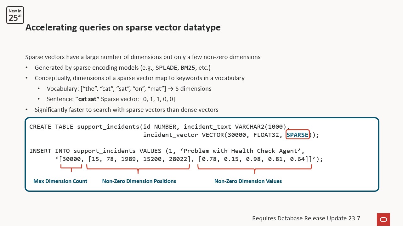
Last, but not least, SPARSE vectors typically have a very large number of possible dimensions, but often only a small proportion of these dimensions have a value assigned. Generated by embedding models such as SPLADE and BM25, SPARSE vectors lend themselves to keyword or vocabulary-based AI workloads. For example, if the Exadata documentation is embedded with one of these models and the total number of dimensions is set to, say, 30,000 (each corresponding to a keyword), each nonzero dimension represents the count of occurrences for that keyword. Dimensions that are not assigned a value by the embedding model are not stored in the vector. Storing only the non-zero value dimensions significantly reduces the size of such vectors and accelerates AI Smart Scan queries.
Combining AI vector similarity search and relational business data
Oracle Database has long been a multi-model database. In recent years, it has been described as a converged database because of its ability to store and process many styles of data and workloads simultaneously and in combination. AI Vector Search exemplifies this strategy by combining vector similarity search with existing Oracle data.
For example, a property search application may use a table that stores ZIP code, asking price, a vector embedding the property’s photo description, and other related data.
CREATE TABLE houses (id NUMBER, zipcode NUMBER, price NUMBER, description CLOB, description_vector VECTOR(1024, FLOAT32));
To query this data efficiently, an index would be created on the description_vector column. There are two main types of indices applicable to vectors. The In-Memory Neighbor Graph vector index, also known as a Hierarchical Navigable Small World (HNSW) index, and the Neighbor Partition Vector index, or Inverted File Flat (IVF_FLAT) index. Additional information about these index structures, including a third type, the Hybrid Vector Index, is available in the AI Vector Search documentation.
AI Smart Scan works transparently with Neighbor Partition Vector (IVF_FLAT) indexes to accelerate queries.
In this example, a Neighbor Partition Vector index is created on the description_vector column.
CREATE VECTOR INDEX house_idx ON houses (description_vector) ORGANIZATION NEIGHBOR PARTITIONS;
To query this table, you might execute SQL such as:
SELECT price FROM houses t
WHERE price < 2000000 AND zipcode = 94065
ORDER BY VECTOR_DISTANCE(description_vector, :query_vector)
FETCH APPROX FIRST 10 ROWS ONLY;
In this query, the goal is to find the 10 most similar properties in the houses table to a reference vector, with prices below a specified amount and within a given ZIP code. What is happening under the covers? Let’s examine the explain plan.
--------------------------------------------------------------------------------------------------------
| Id  | Operation                         | Name                                                       |
--------------------------------------------------------------------------------------------------------
|   0 | SELECT STATEMENT                  |                                                            |
|   1 |  VIEW                             |                                                            |
|   2 |   NESTED LOOPS                    |                                                            |
|   3 |    VIEW                           | VW_IVPSR_11E7D7DE                                          |
|*  4 |     COUNT STOPKEY                 |                                                            |
|   5 |      VIEW                         | VW_IVPSJ_578B79F1                                          |
|*  6 |       SORT ORDER BY STOPKEY       |                                                            |
|   7 |        NESTED LOOPS               |                                                            |
|   8 |     VIEW                          | VW_IVCR_B5B87E67                                           |
|*  9 |      COUNT STOPKEY                |                                                            |
|  10 |       VIEW                        | VW_IVCN_9A1D2119                                           |
|* 11 |        SORT ORDER BY STOPKEY      |                                                            |
|  12 |         TABLE ACCESS STORAGE FULL | VECTOR$VIDX_IVF$32281_32286_0$IVF_FLAT_CENTROIDS           |
|  13 |     PARTITION LIST ITERATOR       |                                                            |
|* 14 |      TABLE ACCESS STORAGE FULL    | VECTOR$VIDX_IVF$32281_32286_0$IVF_FLAT_CENTROID_PARTITIONS |
|  15 |    TABLE ACCESS BY USER ROWID     | HOUSES                                                     |
--------------------------------------------------------------------------------------------------------
The key entries in the explain plan here are IDs 12, 14, and 15. 12 and 14 tell us that AI Smart Scan is being used to offload the vector search to Exadata storage servers and scan the house_idx index. Neighbor partition vector indexes consist of a partitioned table that stores the vector entries (in this example, “VECTOR$VIDX_IVF$32281_32286_0$IVF_FLAT_CENTROID_PARTITIONS”) and another table that represents the centroid, or anchor vector, for each partition (“VECTOR$VIDX_IVF$32281_32286_0$IVF_FLAT_CENTROIDS”).
While the AI similarity search uses the vector index for performance, filtering on price and ZIP code still incurs additional I/O. ID 15 in the explain plan shows that additional I/O, specifically single block reads, are performed on the ‘houses’ table.
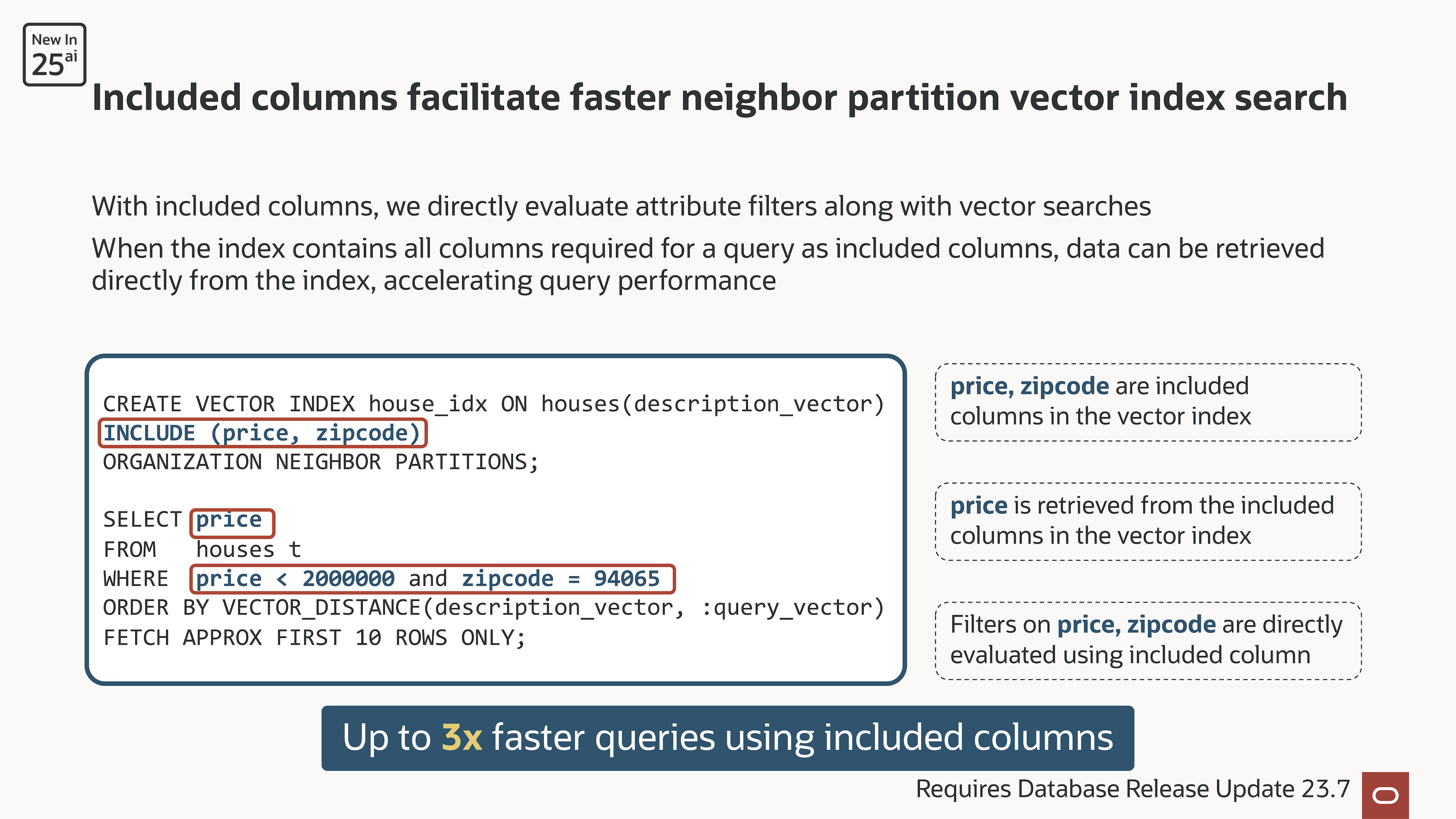
New in the 23.7 release update (January 2025), it is possible to include additional columns in the vector index we created earlier. Called Included Columns in Neighbor Partition Vector Indexes, this capability solves the issue of additional I/O observed in the previous example.
By recreating the index and including the price and ZIP code columns, single block reads can be avoided altogether for the query.
CREATE VECTOR INDEX house_idx ON houses(description_vector)
INCLUDE (price, zipcode)
ORGANIZATION NEIGHBOR PARTITIONS;
The revised explain plan reveals a more streamlined query execution, with TABLE ACCESS BY USER ROWID on the “houses” table eliminated.
----------------------------------------------------------------------------------------------------------
| Id  | Operation                           | Name                                                       |
----------------------------------------------------------------------------------------------------------
|   0 | SELECT STATEMENT                    |                                                            |
|   1 |  VIEW                               |                                                            |
|   2 |   VIEW                              | VW_IVPSR_11E7D7DE                                          |
|*  3 |    COUNT STOPKEY                    |                                                            |
|   4 |     VIEW                            | VW_IVPSJ_578B79F1                                          |
|*  5 |      SORT ORDER BY STOPKEY          |                                                            |
|   6 |       NESTED LOOPS                  |                                                            |
|   7 |        VIEW                         | VW_IVCR_B5B87E67                                           |
|*  8 |     COUNT STOPKEY                   |                                                            |
|   9 |      VIEW                           | VW_IVCN_9A1D2119                                           |
|* 10 |       SORT ORDER BY STOPKEY         |                                                            |
|  11 |        TABLE ACCESS STORAGE FULL    | VECTOR$VIDX_IVF$32281_32305_0$IVF_FLAT_CENTROIDS           |
|  12 |        PARTITION LIST ITERATOR      |                                                            |
|* 13 |         TABLE ACCESS STORAGE FULL   | VECTOR$VIDX_IVF$32281_32305_0$IVF_FLAT_CENTROID_PARTITIONS |
----------------------------------------------------------------------------------------------------------
The inclusion of additional columns in the vector index, coupled with AI Smart Scan’s offload capabilities, can accelerate queries by up to 3x.
Recap
We’ve covered a lot of ground in this post, including: the fundamentals of Exadata AI Smart Scan, which offloads and accelerates AI Vector Search onto Exadata storage servers; Adaptive Top-K Filtering, which quickly and efficiently reduces the amount of data sent to the database servers for further processing; BINARY and SPARSE vector optimizations, which accelerate queries, reduce storage usage, and maintain high accuracy; vector distance column projection, where AI Smart Scan sends the computed distance back to the database server to avoid precomputation and reduce network traffic; and, finally, including business data in neighbor partition vector indexes to eliminate unnecessary I/O and accelerate queries. This is just the beginning of AI capabilities in Oracle Database and Exadata. Additional capabilities will be added here as they are released, so please check back for updates.