Behind the Scenes: GPU Power Smoothing for Large-Scale AI Training

A Tiny GPU Heartbeat for Smoothing AI Power Spikes

GPUs can draw a lot of power. At scale, peak power draw is only part of the challenge. The harder problem is sudden, synchronized changes in power. Bulk-synchronous training can make thousands of GPUs pause and resume together, producing sharp transitions that stress transformers, power distribution units, and even upstream turbine generators.

While there has been several approaches to smooth these fluctuations, we present a novel and fast software solution. We introduce AET (Average Elapsed Time), a millisecond-scale GPU heartbeat that provides an ultra-fast, accurate GPU activity signal for our smoothing process.

When you run a training job on a single GPU, power is mostly “somebody else’s problem.” You might notice your workstation get louder and warmer, but you probably won’t think about the data center’s power limits.

Now scale that job to tens of thousands of GPUs. Suddenly that “somebody else” turns into a real person: the on-call facilities engineer staring at the power trace, mildly annoyed about being paged. A moment later the escalation hits: your phone starts ringing while Slack fills up with the kind of “Is this your job?” DMs that are clearly not a real question.

Modern large-scale training is often bulk‑synchronous. GPUs spend some time computing, then hit synchronization points like collective operations (for example, “All‑Reduce”). While they wait for the slowest rank, many GPUs briefly go idle.

Take a look at the plot below (Figure 1): on a single GPU, a bulk‑synchronous workload can look like a square wave (compute, pause, compute, pause), with power jumping up and down like a switch.

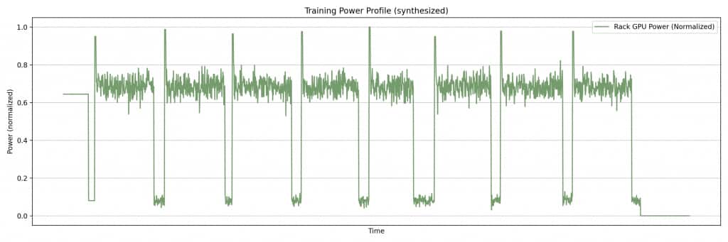
Those rapid changes can stress transformers, UPS devices, and power distribution units (PDUs), and can trip upstream protections. On a large, bulk-synchronous training job, those synchronized power fluctuations stack up across co-located nodes. You end up seeing the same signature at the rack level, then the data center level, and eventually at the utility interconnect.

At OCI scale, those swings can reach tens or even hundreds of megawatts. If the oscillation’s frequency content lines up poorly with resonant characteristics of grid components (for example, turbine generators or long transmission lines), it can create real stability concerns and even mechanical risk.

To stay on the safe side, operators often cap GPU max power and run the facility more conservatively than they would like until they are confident a job’s power profile is well-behaved. If you are a cloud provider, that conservatism is expensive; if you are renting GPUs, it shows up as higher costs or lower performance. Either way, the square wave eventually hunts you down and finds its way into the business, as either an invoice line item or a throughput graph that makes everyone frown in the team meeting.

Ideally you want a smooth power profile that stays within facility and grid requirements. This is exactly the kind of problem that keeps a lot of people awake at a cloud provider like Oracle.

Since this is a relatively new problem, there is not a single standard, perfect way to mitigate it yet. Hardware power‑smoothing techniques exist, but they can be expensive, slow to roll out, and hard to validate fleet-wide. Some newer NVIDIA racks include built-in power-smoothing features, but those have a finite service life (one to two years, depending on usage) and are not a practical long-term answer.

At OCI, we adopted several approaches, including the software approach described here, which we could deploy and validate quickly against real training jobs on the machines we already had.

The Software Solution: Fill the Valleys, Back Off on the Peaks

The idea is almost too simple: run a second, cooperating process alongside the training job that watches for short idle gaps on the GPU.

• When training goes quiet for a moment, the secondary process quickly injects a tiny workload on the GPU to fill the dip.
• The moment the primary workload needs the GPU again, the secondary process gets out of the way and yields.

If you do this well, sharp power drops disappear, without significantly affecting the training workload.

Ideally the secondary work is useful, but in practice we bias toward work that starts and stops cleanly (short, dense math like small GEMMs). The hard part is not the math; it’s knowing, right now, whether the GPU is actually idle.

Latency Is Not Your Friend

If you want software to smooth power, the timing is unfairly against you. You should  react quickly enough that the grid and facility monitoring barely notice. That means detecting the moment the primary workload goes quiet, within milliseconds, so you can start filling the dip before upstream protections see a sharp power drop. Then you need to notice just as quickly when the primary comes back, so you can get out of the way before you create contention.

If your “GPU went idle” indicator arrives tens of milliseconds late, you miss most of the valley; if your “GPU is busy again” indicator lags on the way back up, you step on the training job’s toes and degrade throughput. Even a 5% slowdown on a training run that lasts hundreds of days can be too long and expensive, and it tends to make impatient stakeholders unhappy.

Standard telemetry like NVIDIA’s NVML power/utilization is useful, but it is not usually built for sub‑20 ms control loops. The sampling and reporting cadence can be on the order of tens of milliseconds, and it is hard to tell whether “busy” is coming from training or from the smoother.

The goal, then, is a feedback loop that can react within a few milliseconds in both directions (Busy→Idle and Idle→Busy), so the secondary can fill power valleys and still yield instantly when the model needs the GPU.

To meet that requirement, we created AET (Average Elapsed Time): a tiny GPU heartbeat that lets a secondary process react in a few milliseconds, smoothing square-wave valleys without slowing down the primary training job.

AET: A Tine GPU Heartbeat

AET is a lightweight probe for measuring the GPUGPU activity. We periodically enqueue a tiny, near no‑op kernel on a low‑priority CUDA stream, then measure the elapsed time from launch to completion, including queueing and dispatch. 

• Busy GPU: the probe waits behind the primary job and returns more slowly. 

• Idle GPU: the probe sees little queuing and returns quickly. 

That single number (elapsed time) becomes a fast proxy for “how busy is the GPU right now?” 

In practice, we continuously run this heartbeat, and the control loop sees Busy→Idle and Idle→Busy transitions on the order of a few milliseconds. That’sThat is fast enough to start filling a valley before facility telemetry shows a sharp edge, and to stop before we steal meaningful time from training. 

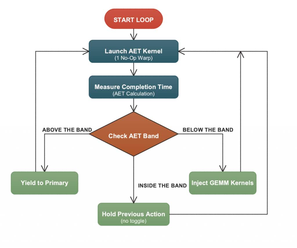
Figure 2 summarizes the control loop at a high level: use AET as the fast activity signal, inject secondary work during idle periods, and yield immediately when the primary becomes active. 

A Simple Way to Make Decisions Fast: the AET Band

A notable feature of AET is precise yielding: we can detect contention and yield within a few milliseconds. Without AET, one would have to periodically back off and check native GPU telemetry (for example, NVML power) to infer whether the primary has become active again.

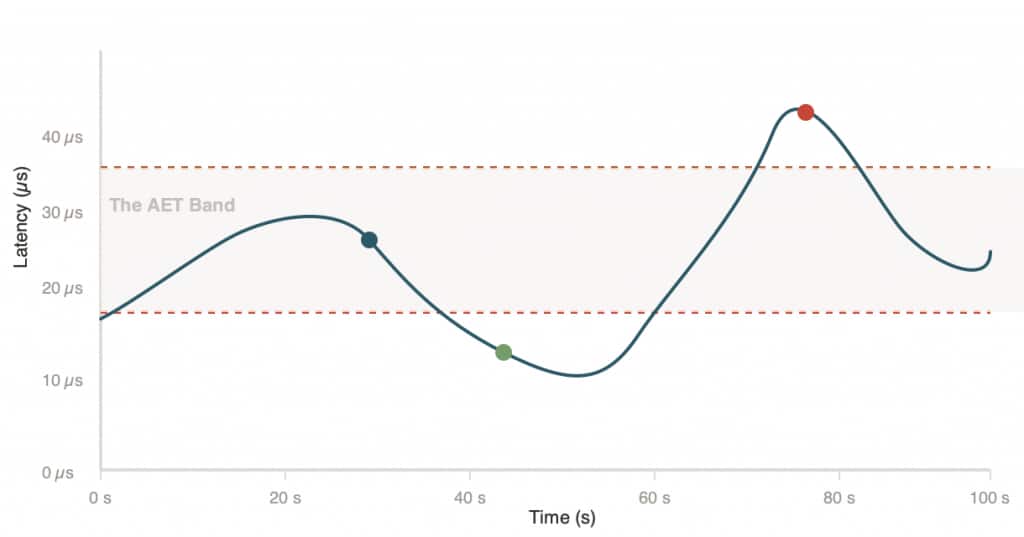
To make this fast signal easy to act on, the control loop maps the (smoothed) AET time series into a three‑zone “band” using two thresholds:

• Below band (idle): inject secondary work.
• Within band (active): hold steady.
• Above band (contention): yield immediately.

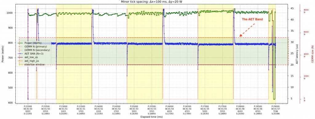
Figure 3 visualizes these three regions of the AET band and how the thresholds map the (smoothed) AET signal into simple “inject/hold/yield” decisions.

In our experience, a sustained above‑band AET spike is a strong sign that the smoother is colliding with the primary (real contention), so the secondary backs off immediately.

This is also why AET works better than periodic polling. We do not have to pause and “probe” for activity. Above‑band latency gives us a direct, millisecond‑scale signal that the secondary is getting in the way.

Co-Residency with Training: NVIDIA MPS

We co-locate the training job and a cooperating power-smoothing process on the same GPU using NVIDIA MPS (Multi-Process Service). MPS lets multiple processes share one GPU efficiently, avoiding the context switching and serialization overhead you often get with naïve multi-process GPU use.

The rule is simple: the secondary should back-off as soon as the primary needs the GPU. When AET says “idle,” the secondary injects work. When AET says “busy” (or we detect contention), the secondary yields immediately.

Done right, the smoother mostly uses cycles that would otherwise be low activity, so the throughput impact on training stays negligible.

Figure 4 illustrates how MPS enables this co-residency: the secondary can run in the gaps, but it backs off as soon as the primary needs the device.

Figure 5 shows the result on a synthetic workload. The unshaded regions are where the primary workload is running normally. When the primary’s activity drops (an idle valley), the AET heartbeat (blue) drops quickly. The controller detects that Busy→Idle transition and enables the smoother. In the shaded (yellow) regions, the smoother injects secondary work to fill the valley. When the primary resumes, AET rises rapidly (Idle→Busy) and the smoother yields immediately. As a result, the green power trace stays relatively stable across the primary’s active/idle transitions in both the unshaded and yellow-shaded regions.

From a Noisy Signal to Production-ready AET

Raw AET measurements are fast. The probe kernel itself is tiny, and on a quiet GPU an end‑to‑end probe can complete in tens of microseconds. But a fast signal is not automatically a clean signal.

GPU scheduling is jittery, and AET reflects more than just kernel execution latency. It also picks up CPU‑side launch timing, driver and queueing delays, PCIe traffic, and changes in GPU clocks and power states.

In practice, that variability shows up as measurement noise. The biggest contributors tend to be:

• Driver/API overhead: every kernel launch and event timestamp has CPU/driver overhead.
• GPU P‑states / DVFS: these are GPU power/clock states. When the GPU has been idle, it may downclock, so the same “no-op” probe can take longer even without any new contention.
• Bus contention: DMA-heavy activity can compete for shared bandwidth and delay dispatch.
• OS noise: if the CPU thread launching probes is preempted by interrupts or background work, the gaps between launches can widen, and the timing becomes noisier.

To make AET production‑useful, we clean it up with simple statistical and systems techniques:

• Batch multiple probes per sample and use an average or trimmed average to reduce single‑probe jitter.
• Smooth the time series with a short moving average (for example, a small EMA) to suppress outliers without adding too much lag.
• Time‑box each probe by capping the maximum wait, so the sampling period stays predictable even when the GPU is busy.
• Prioritize the sampling loop on the CPU, so it is less likely to be delayed by OS scheduling.
• Normalize for DVFS/P‑state changes by dividing AET by GPU clock frequency; this reduces sensitivity to downclocking.

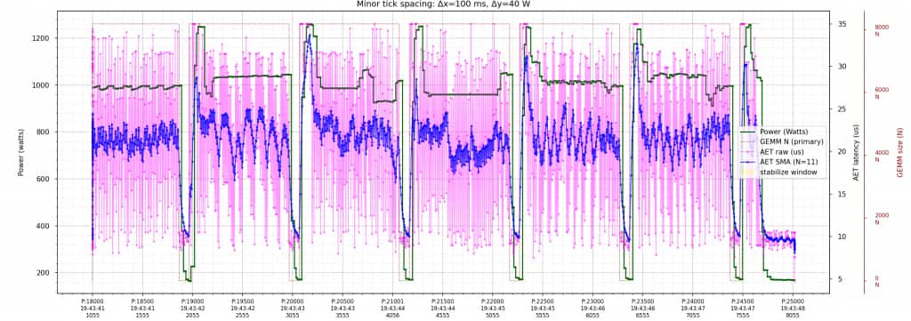
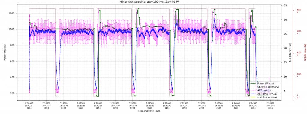
The two plots below (Figures 6 and 7) show the effect of batching and smoothing on the AET signal. With fewer probes per sample, the measurements are visibly noisier; with more probes per sample, they are cleaner, and the same short EMA keeps transition latency low.

Keeping the Heartbeat Predictable: A Designed Sampling Period

The slightly unintuitive part of AET is that the thing you measure (probe latency) can also slow down your measurement loop. When the GPU is slammed, probes naturally take longer to complete. In other words, we needed an SLA on how quickly we could produce each cleaned sample.

The trick is time‑boxing. We put a hard cap on how long we will wait for each probe to finish (for example, by bounding the event wait). If a probe has not been completed by the cap, we stop waiting, record it as “capped,” and move on. At that point, the GPU is busy enough that we are already seeing contention, and the exact extra delay does not change the controller’s decision. This gives us a hard upper bound on how long it takes to produce each aggregated sample.

As a concrete example, imagine we build each sample from 100 probes. Suppose we know that an AET of ~20 µs already indicates contention between the primary and secondary. We can then cap each probe at a slightly higher, round number—25 µs. Once we are above the contention threshold, the exact value does not change the controller’s decision. The cap simply bounds how long each probe can take, so we can produce each sample faster and keep the sampling cadence predictable.

In the worst case, the GPU is saturated, and every probe hits the cap, so the whole batch still finishes in ≤ 2.5 ms. This provides an upper bound on the heartbeat interval.

Then we apply a short EMA (for example, an effective window of ~5 samples) to reduce noise without hiding quick transitions. You can think of this like a small sliding window. It costs only a few samples of lag, not tens of milliseconds.

In practice, Busy→Idle and Idle→Busy changes show up within a couple of new samples. With a worst‑case sample interval of ≤ 2.5 ms, that means the control loop reacts within roughly 2 samples, which would be about 5 ms.

Other Challenges and Caveats

• Activity ≠ power: AET measures contention/queueing, not watts. It is a timing signal, not a direct readout of board power. A GPU can look “active” and still draw very different watts depending on clocks, power caps, and the specific kernels in flight.
  
  • Mitigation: we use AET as the fast signal for when to inject and when to yield (the AET band), then validate the resulting power behavior with slower, direct measurements. When we need tighter correlation, we pair AET with auxiliary signals (for example clocks, power-cap state, and delayed NVML power) to improve power prediction without putting NVML in the critical control loop.
    
• CPU overhead and multi‑GPU scaling: each GPU needs a fast sampler loop. The heartbeat is cheap, but it is not free: launching kernels and collecting timestamps has CPU and driver overhead, and it scales with device count. If you try to multiplex too many GPUs on one thread, the sampling cadence can slip, and the control loop becomes less responsive.
  
  • Mitigation: we keep the probe kernel minimal, the sampling loop lightweight, and we dedicate a small, high‑priority thread per GPU, so each GPU maintains a predictable millisecond‑scale cadence.
    
• Machine‑dependent thresholds: ideal AET bands vary by GPU, driver, and configuration. “Good” below/within/above thresholds depend on details like GPU model, firmware/driver versions, MPS settings, and even how clocks behave under idle and bursty load. A single set of constants can work poorly when moved across a heterogeneous fleet.
  
  • Mitigation: we calibrate per machine (or per hardware SKU) to pick below/ within/above thresholds, then use those calibrated bands in the fast path.

How this Fits into the Broader Industry Effort

This problem is actively being worked on across the cloud and hyperscale ecosystem, and versions of it have been discussed publicly.

Getting smooth, millisecond‑scale control without harming training throughput is non‑trivial: signals are noisy, attribution is ambiguous, and hardware and driver behavior varies across fleets.

Given that, our AET‑based approach is best viewed as a software complement to hardware smoothing. It is lightweight to roll out, and in our evaluation, it was effective at reducing power fluctuations with minimal performance degradation.

Conclusion

At Oracle/OCI scale, during large training runs with tens of thousands of GPUs, “small” millisecond‑level power fluctuations stop being a local GPU detail and turn into a facility problem.

Smoothing that behavior at this scale is non‑trivial, and in practice it needs a multi‑layer approach across hardware and software. It also takes coordination across the cloud provider, the customer running the job, the GPU vendor, and the utility provider.

Average Elapsed Time (AET) is our software piece: a tiny, low‑priority GPU heartbeat that makes short‑timescale contention visible fast enough for a cooperating process to fill brief power drops, then yield immediately when training needs the device.