

Customers are increasingly adopting ML-driven applications—such as semantic search, recommendations, and RAG—that rely on vector search. Compared to traditional keyword search, vector workloads have different and often higher demands on CPU, memory, and storage/IO. In the absence of clear sizing guidance, many deployments are under-provisioned or scaled using trial-and-error, leading to poor latency, low throughput, instability under variable workloads, and costly rework during production rollout. This document provides practical OpenSearch vector search sizing guidelines to help teams estimate capacity upfront and provision clusters that meet performance and reliability requirements as data and query volumes grow.
Technical Background of Vector Search
What is vector search?
Vector search finds items that are semantically similar (in meaning) by comparing numeric vectors (“embeddings”) representing text, images, audio, etc. Instead of exact keyword matches, it retrieves the nearest vectors to a query vector using a similarity metric (e.g., cosine similarity, dot product, L2 distance). In other words, given a query vector, we retrieve the k nearest neighbours (KNN)—which correspond to the most semantically similar items.
Why not brute-force KNN?
A conventional exact k-nearest neighbours (KNN) search compares the query vector against every vector in the dataset, which is O(n) per query—often too slow and costly at scale. To improve query speed, approximate nearest neighbour (ANN) algorithms are commonly used.
How does HNSW help?
HNSW (Hierarchical Navigable Small World) is an ANN method that significantly reduces query time by searching a graph-based index rather than scanning all vectors. It builds a multi-layer graph where vectors are nodes and edges connect “nearby” vectors; query-time search navigates this graph to quickly reach good candidates (trading a small amount of recall for large latency/throughput gains). The internal details of HNSW algorithm are out of scope for this document. However, it is recommended to study the internal details of the algorithm for a better understanding of this document.
This blog provides a lucid and visual explanation for the same: https://www.pinecone.io/learn/series/faiss/hnsw/
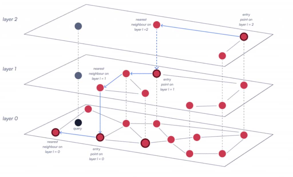
Opensearch supports IVF and HNSW algorithms, this blog focuses on HNSW algorithm and provides sizing recommendations for the same.
Common HNSW Parameters
- m: Max number of connections (neighbours) per node in the graph.
- Higher M → better recall, higher memory usage, slower indexing.
- ef_construction: Controls search breadth during index (graph) construction.
- Higher ef_construction → better index quality/recall, slower indexing and more resource use.
- ef_search: Controls search breadth during queries.
- Higher ef_search → better recall, higher query latency and CPU.
Vector Search in Opensearch
OpenSearch stores data in indices. Each index is partitioned into shards—primary shards for writes and replica shards for redundancy and read scaling. Each shard is effectively a Lucene index.
Within a Lucene index, data is written into immutable segments. Over time, segments are merged into larger segments to improve search efficiency. For vector search, each segment has its own HNSW (Hierarchical Navigable Small World) graph, which acts as the ANN index for the vectors in that segment.
In common vector-search ingestion patterns (bulk/one-time ingestion followed by mostly read/query traffic), segments typically converge via merges. Once merges have largely settled, a shard would be containing:
- the shard’s documents/vectors, and
- one (or a small number of) HNSW graph(s) representing the final segment set.
Importantly, each shard builds and maintains its own HNSW graph(s)—so total memory and compute requirements scale with the number of shards (primaries + replicas).
Unlike traditional keyword search, vector search performance depends heavily on fast random access to both the HNSW graph and the underlying vector/document data. To enable this, OpenSearch/Lucene relies on off-heap memory (via memory-mapped files / native memory) to keep:
- HNSW graph structures, and
- open segment files used during ANN traversal readily accessible.
This makes off-heap capacity a primary sizing factor for vector workloads: clusters must be sized and configured with sufficient off-heap headroom to hold HNSW graphs and associated files for all active shards (including replicas). This directly informs the next section on sizing guidelines (node memory sizing, shard strategy, and headroom planning).
Sizing Guidelines
A sizing calculator has built as an excel spreadsheet, that can be downloaded at this link. It is intended to be used as an interactive calculator: you enter workload-specific inputs, optionally tune a few assumptions, and the sheet produces recommended OpenSearch cluster sizing outputs (shards, nodes, memory, CPU, and storage) for data nodes of the cluster.
1) Fill in the Known Inputs (customer/workload specific)
Update these fields first:
- Vector dimension (d): dimension of vector created by the selected embedding model (e.g., 768).
- Number of documents (doc): number of documents in the dataset.
- Number of chunks (c): number of chunks or vectors created by each document.
- m (HNSW parameter): graph connectivity parameter (commonly 16 by default in many setups).
- Replica shards per primary: for HA and read scale (often 1).
These values drive the total HNSW memory footprint and total data volume.
2) Review and (optionally) tune the Tunable Parameters
These are “knobs” you can adjust based on performance goals, operational constraints, and cost:
- HNSW graph size per shard (GB): target HNSW graph footprint per shard (often ~10–30 GB).
Smaller per-shard graphs generally improve latency but increase shard count. - Ratio of shard size / graph size: multiplier to estimate full shard size from the HNSW graph size.
Use ~1.8 as a starting point for “one vector per document with minimal extra fields”; increase it if documents have additional fields or multiple vectors. - Number of shards per data node (primary + replica): Impacts parallelism and node count.
Less number of shards/node can improve performance by parallelising the workload, but lead to larger number of nodes. - Ratio of memory to OCPUs: used to derive CPU from memory.
A higher ratio reduces CPU (lower cost) but may limit throughput under concurrency. - Safety buffer for total memory (%): headroom to absorb spikes, merges, OS overhead, etc.
- Safety buffer for storage (%): additional storage headroom; also helps provision higher IOPS where storage performance scales with volume.
Users should generally start with the defaults, then adjust based on measured latency/throughput targets and operational limits (max shards, max nodes, etc.).
3) Read the Derived Outputs (recommended sizing)
Once inputs/assumptions are set, the spreadsheet computes:
- Number of vectors (n): total vectors to be indexed. Product of number of documents and number of chunks (doc * c).
- Total HNSW graph size (primaries only): estimated memory footprint of the graph(s) for all primary shards.
- Total data size (primaries only): estimated on-disk primary data size using the shard-to-graph ratio.
- Total data size (primaries + replicas): accounts for replication factor.
- Shard size (GB): derived from “graph size per shard × shard/graph ratio”.
- Total number of primary shards: total primary graph footprint divided by target graph size per shard (rounded up).
- Off-heap memory per data node: sized to keep shard data/graph files readily accessible for vector search.
- Total memory per data node: derived from off-heap, assuming a 50/50 heap vs off-heap split.
- Number of data nodes: derived from total shards and target shards per node (rounded up).
- OCPUs per data node: derived from memory per node and the memory:CPU ratio (rounded up).
- Block storage per data node: per-node storage allocation including storage buffer, rounded to a convenient increment.
4) Iterate until the sizing matches your constraints
Vector search sizing usually needs a few rounds of iteration rather than a single right-sized configuration from the start. The most effective approach is to begin with a reasonable baseline, review benchmark and cluster results, and then tune separately for ingestion and search depending on the bottleneck.
- Start below the node limit: If the estimated node count is too high, increase graph size per shard and/or shards per node first. Since OCI OpenSearch supports up to 100 data nodes, it is best to start below that limit so there is still headroom to scale.
- Use benchmark results to drive the next step: After each run, review latency, recall, error rate, and cluster metrics together. If latency is not acceptable, these signals help identify whether the bottleneck is compute, memory, indexing pressure, merges, or search configuration.
- Optimize ingestion separately: Ingestion generally requires higher OPCUs and benefits from minimizing replicas during load, along with tuning settings such as refresh interval and translog sync to reduce indexing overhead.
- Treat search tuning as a separate loop: Search optimization is usually more complex because it depends on graph size, shard count, ANN parameters such as m and ef, and the nature of the queries themselves. Tuning search therefore requires careful review of these parameters together with benchmark results such as latency, recall, and error rate.
Sample Results
Tests were run based on the OpenSearch Benchmark cohere-10m dataset, which is the 10 million-vector subset of the cohere-wikipedia-22-12-en-embeddings corpus in the official vectorsearch workload and is provided in HDF5 format for benchmarking. OpenSearch’s published benchmark configuration for the corresponding Cohere 10m Dataset dataset describes it as a 768-dimensional inner-product workload with a 10,000-query evaluation set, making it a useful large-scale dataset for vector search sizing and search-quality evaluation.
For this study, a shard size of 10 GB and 2 shards per node was used to prioritize search and ingestion quality, and the benchmark was run across three OCI shapes: E3, E4, and E5. In OCI, a shape defines the OCPU, memory, and related resources allocated to an instance, and flexible shapes allow these resources to be tuned within supported limits. In our results, this progression is reflected in the improved performance as we move from the older shape to the newer one. Enough buffer has been inculcated in the sizing calculations to ensure the cluster stays stable and is reslient to any spikes in loads.
Test Config
Below is the configuration of the test with the cohere 10m dataset and default opensearch benchmark configurations.
| Parameter | m | ef | Dataset | Dimension | Ingestion Clients | Search Clients | Search Queries |
|---|---|---|---|---|---|---|---|
| Value | 1 | 256 | Cohere 10m | 768 | 8 | 8 | 10,000 |
Input Config to Sizing Calculator
Below are the inputs provided to the sizing calculator, based on the above test configuration:
| Input Parameter | Value | Reasoning |
|---|---|---|
| Number of documents | 10,000,000 | Cohere 10m dataset |
| Chunks per document | 1 | 1 vector per document |
| Shard size | 10 GB | Lower for optimal search results |
| Shards per node | 2 | Lower for optimal search/ingestion results |
| OCPU: Memory Ratio | 1:6 | Higher OCPUs used for better ingestion performance |
Derived Cluster Config
Following is the cluster config found:
| Parameter | Number of nodes | OCPU per node | Memory per node | Storage per node |
|---|---|---|---|---|
| Data Nodes | 4 | 15 | 90 GB | 300 GB |
| Master Nodes | 1 | 4 | 20 GB | NA |
Results
These are the results of the tests run for clusters with different shapes.
| Shape | Ingestion Latency P90 | Ingestion Latency p99 | Search Latency p90 | Search Latency p99 | Mean recall@k |
| VM.Standard.E3.Flex | 1790 ms | 3500 ms | 56 ms | 105 ms | 0.99 |
| VM.Standard.E4.Flex | 200 ms | 1500 ms | 67 ms | 84 ms | 0.99 |
| VM.Standard.E5.Flex | 78 ms | 804 ms | 65 ms | 78 ms | 0.99 |
Tuning
Metrics: CPU
Detecting a CPU bottleneck is an important part of vector search sizing because both ingestion and search can become CPU-bound due to graph construction, ANN traversal, segment merges, scoring, and other background processing. Sustained high CPU utilization, increased load, rising thread-pool queues or rejections, and worsening latency without corresponding memory or disk pressure are common indicators that the workload is constrained by CPU. In such cases, increasing CPU capacity, for example by moving to a larger shape or increasing available OPCUs, can improve indexing throughput, reduce search latency and tail latency, lower queueing and error rates, and provide additional headroom for background tasks. As with other sizing changes, this should be validated against cluster metrics to confirm that CPU is the primary bottleneck and that the improvement is not being limited by memory, storage, or shard-layout constraints. In the example below, it can be seen that increasing the number of CPUs after identifying the bottleneck led to significant improvements in the benchmark results.
| Cluster Config | Ingestion Latency (p99) | Search Latency (p99) | Cluster CPU |
|---|---|---|---|
| 4 Data Nodes, 10 OCPU/node, 90 GB RAM/node, E3 Flex | 9.9 sec | 104 sec | At 100% |
| 4 Data Nodes, 15 OCPU/node, 90 GB RAM/node, E3 Flex | 869 ms | 105 ms | Around 60–70% |
Metrics: Latencies
Ingestion latency can often be improved significantly by reducing background indexing overhead during bulk-load phases. In this case, the following settings were used to optimize ingestion performance.
- refresh_interval: -1
- translog.durability: async
- translog.sync_interval: 30s
Setting refresh_interval to -1 avoids periodic refreshes while ingestion is in progress, which reduces the cost of making newly indexed documents searchable during the load phase. Configuring translog.durability as async and increasing translog.sync_interval to 30s reduces the frequency of translog fsync operations, lowering write overhead and improving ingestion throughput and latency.
These settings are particularly useful when the workload is ingestion-heavy and immediate searchability is not required during the load phase. The results shown below reflect the impact of these changes and demonstrate the corresponding improvement in ingestion latency.
| Test Mode | Ingestion Latency (p90) | Ingestion Latency (p99) | Search Latency (p90) | Search Latency (p99) | Recall @ k |
|---|---|---|---|---|---|
| Without Optimization | 200 ms | 1500 ms | 67 ms | 84 ms | 0.99 |
| With Optimization | 120 ms | 220 ms | 59 ms | 71 ms | 0.99 |
Node Count
OCI OpenSearch currently recommends up to 100 data nodes, so sizing should generally begin below that limit in order to leave enough headroom for future scaling and iteration. If the initial estimate exceeds this limit, the first step is usually to increase the graph size per shard and/or the number of shards per node.
For example, for a dataset of 2,000,000,000 vectors, using the minimum recommended shard size of 10 GB may result in an estimated 164 nodes; increasing the shard size to 20 GB or raising shard density to 16 shards per node can reduce the requirement to roughly 82 nodes, providing a more practical starting point with room for experimentation.
Upcoming Optimization (Planned for End of August 2026): AVX V2 512:
As part of an upcoming release planned for the end of August, OCI OpenSearch will introduce support for AVX-512 (Advanced Vector Extensions 512) on supported compute shapes.
Modern CPUs that support AVX-512 (Advanced Vector Extensions 512) can significantly accelerate vector similarity computations by processing multiple vector dimensions in parallel using wide SIMD (Single Instruction, Multiple Data) instructions. OpenSearch’s FAISS engine leverages these instructions to optimize both indexing and query execution, particularly for high-dimensional embeddings. This is enabled by default if using the shape : E5 Flex.
For vector search workloads, enabling AVX-512 typically results in lower query latency, higher throughput, and better CPU utilization, allowing each data node to serve more queries before becoming CPU-bound. While AVX-512 does not reduce the HNSW index size or native memory requirements, it increases the effective compute capacity of each node, which can translate into fewer nodes required to achieve a given latency target.
Below table depicts the huge improvment seen in both ingestion and search latency with AVX enabled instances.
| Config | Cluster Config | Ingestion Latency (p99) | Search Latency (p99) |
|---|---|---|---|
| AVX-512 Disabled | 4 Data Nodes, 15 OCPU/node, 90 GB RAM/node, E5 Flex | 804 ms | 78 ms |
| AVX-512 Enabled | 3 Data Nodes, 4 OCPU/node, 64 GB RAM/node, E5 Flex | 200.39 ms | 13 ms |
Choosing the Right Vector Compression Strategy
As vector datasets grow from millions to billions of embeddings, vector compression becomes essential for balancing search quality, latency, and infrastructure cost. Different compression techniques reduce the memory required to store vectors by representing them with fewer bits, allowing more vectors to fit into memory and improving cache efficiency. However, higher compression typically comes at the cost of lower recall, making the optimal choice dependent on the application’s accuracy and scalability requirements.
More details can be found in John Handlers talk
| Method | Explanation | Trade-offs | Best For |
|---|---|---|---|
| FP32 | Full 32-bit floating-point vectors with no compression. | Recall: Highest Latency: Moderate Infrastructure Cost: Very High | Maximum search accuracy where memory and infrastructure cost are not primary concerns. |
| FP16 | Half-precision floating-point vectors, reducing vector memory by approximately 2×. | Recall: Very High Latency: Good Infrastructure Cost: High | Accuracy-sensitive deployments requiring modest memory savings. |
| SQ8 | 8-bit scalar quantization that provides an excellent balance between memory efficiency and search quality. | Recall: Very High Latency: Very Good Infrastructure Cost: Moderate | Enterprise semantic search and RAG workloads. |
| SQ4 | 4-bit scalar quantization that further reduces vector storage while introducing additional approximation. | Recall: High Latency: Excellent Infrastructure Cost: Low | Large-scale vector search with a focus on reducing infrastructure costs. |
| 16× Compression | Aggressive low-bit quantization that reduces vector storage by approximately 16× (≈10× overall HNSW memory reduction). | Recall: Moderate–High Latency: Excellent Infrastructure Cost: Very Low | Multi-billion vector deployments prioritizing scalability, latency, and memory efficiency. |
| Binary Quantization | Represents each vector dimension using a single bit, providing the highest compression ratio. | Recall: Moderate Latency: Excellent Infrastructure Cost: Lowest | Extremely large ANN deployments where maximum compression is the primary objective, typically with reranking. |
Best Practices
In addition to benchmark results, a small set of operational best practices should be applied when evaluating vector search configurations. These practices help ensure that a configuration that performs well in a benchmark run also retains sufficient stability and headroom under sustained production load.
- Ensure the index is search-ready: Search performance should be evaluated only after segment merges have largely completed, indices have been warmed up, and sufficient memory is available to keep the HNSW graph and associated files readily accessible. Measuring search before the index reaches this steady state can lead to misleading conclusions.
- Optimize ingestion settings for bulk loads: During ingestion-heavy benchmark phases, replica count should be kept at 0, where acceptable, to avoid duplicate indexing work. If search is not required during ingestion, refresh_interval can be set to -1 to reduce refresh overhead. Additional gains may be achieved by tuning translog behavior, for example by using asynchronous durability and a longer sync interval during bulk load, and restoring more conservative settings once ingestion is complete.
- Maintain operational headroom in node sizing: After each benchmark run, cluster metrics should be reviewed to confirm that sufficient headroom remains across CPU, memory, disk, and indexing or search pressure. Even when latency and throughput appear acceptable, a configuration without adequate buffer may still become unstable under sustained workload, traffic spikes, or recovery events.
There could be many more optimisations that can be specific to your use case. The given sizing calculator is meant for the general vector search use case and can help you in at least getting started with a good enough configuration to handle your workloads so that you may focus more on optimisations and iterate faster to the right configuration.