
Load Iceberg tables through the catalog your organization already uses, keep them fast with compaction, clustering and metadata-based statistics, and build bronze, silver and gold layers as one workflow.
Writing Iceberg is the easy part
Apache Iceberg has become the default open table format for the lakehouse. Being able to write an Iceberg table is now table stakes for a data pipeline tool. Two problems are harder, and they decide whether an Iceberg lakehouse works in practice.
The first is the catalog. Every platform has its own: Oracle, Databricks and Snowflake each run one, and many teams also run an open-source catalog. A pipeline tool that writes to only one of them forces you to decide where the data will be consumed before you build the pipeline, and to rebuild it when that changes.
The second is that Iceberg tables degrade. Every commit adds files, small files pile up, related rows end up scattered across files, and the statistics the optimizer relies on go stale after every load. Most teams handle this with a separate set of maintenance jobs, usually Spark, that someone has to write, schedule and watch.
Oracle Data Transforms, the pipeline builder in Autonomous AI Lakehouse, handles both inside the same pipeline:
- Every major catalog. One Apache Iceberg connector writes through Oracle AI Data Catalog, Databricks Unity Catalog, Snowflake Open Catalog (Apache Polaris) or any catalog that implements the Iceberg REST specification.
- Compaction and clustering as workflow steps, so table maintenance runs on the same schedule as the loads that create the need for it.
- Statistics from Iceberg metadata, which are faster than scanning a large share of the data and more accurate than scanning a small sample.
We’ll use one example throughout. A retailer loads order lines from its order management system into an Iceberg table, ORDER_LINES, every 15 minutes. Analysts query it from Autonomous AI Lakehouse, and a data science team works on the same table from Databricks.
Why Data Transforms
Data Transforms is built into Autonomous AI Lakehouse. There is nothing to install, and it covers the whole pipeline in one tool: load data from applications, databases, files and object storage; transform it with a no-code data flow designer or SQL; orchestrate the steps as workflows; schedule them; and monitor every run from one console. Transformations execute inside the Lakehouse, so data is not pulled out to a separate engine and pushed back. The same tool reaches outward too, with connectors for Oracle Fusion, NetSuite, Salesforce and other SaaS applications, the major cloud warehouses and lakehouses, and open formats such as Apache Iceberg. The result is fewer tools, fewer hand-offs between them, and one place to see what ran, what failed and why.
For the lakehouse, that means the load, the table maintenance and the statistics refresh are steps in one workflow, rather than a Data Transforms job, a Spark job and a database job that three people keep in sync.
1. One connector, every catalog
Supported catalog providers
When you create an Apache Iceberg connection in Data Transforms, you choose a Catalog Provider. There are four:
| Catalog provider | What it is | Storage | Authentication |
|---|---|---|---|
| Oracle AI Data Catalog | Oracle’s unified catalog; exposes governed Iceberg namespaces and tables | OCI Object Storage (S3-compatible) | Database user and password |
| Databricks Unity Catalog | The Databricks governance catalog, through its Iceberg REST interface | Azure Data Lake Storage | OAuth (client ID and secret) |
| Snowflake Open Catalog | Snowflake’s managed service for Apache Polaris | Amazon S3 | OAuth (client ID and secret) |
| Generic REST catalog | Any catalog that implements the Iceberg REST specification, such as Apache Gravitino | OCI Object Storage (S3-compatible) or Amazon S3 | None, user and password, or OAuth |
Between them, these cover where most Iceberg data lives today: Oracle’s own catalog, the catalogs of the two largest third-party lakehouse platforms, and the open REST standard that the rest of the ecosystem is converging on.
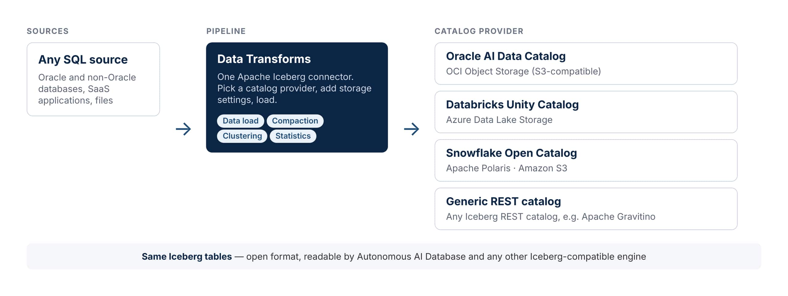
Figure 1. One Iceberg connector in Data Transforms, four catalog providers.
Setting up a connection
Creating the connection takes a few fields:
- Choose the provider. Create a connection of type Apache Iceberg and pick the catalog provider.
- Point to the catalog. Enter the catalog name and the REST URL (or, for Oracle AI Data Catalog, the service URL), along with the credentials for that catalog.
- Add storage settings. Provide the region and keys for the object store that holds the table files.
- Tune if needed. Under Advanced Options, Batch Update Size controls how many records are updated on the target at a time (the default is 5,000).
The connection is then available as a target in a Data Load, so any SQL-based source that Data Transforms can read can be landed as Iceberg tables in that catalog.
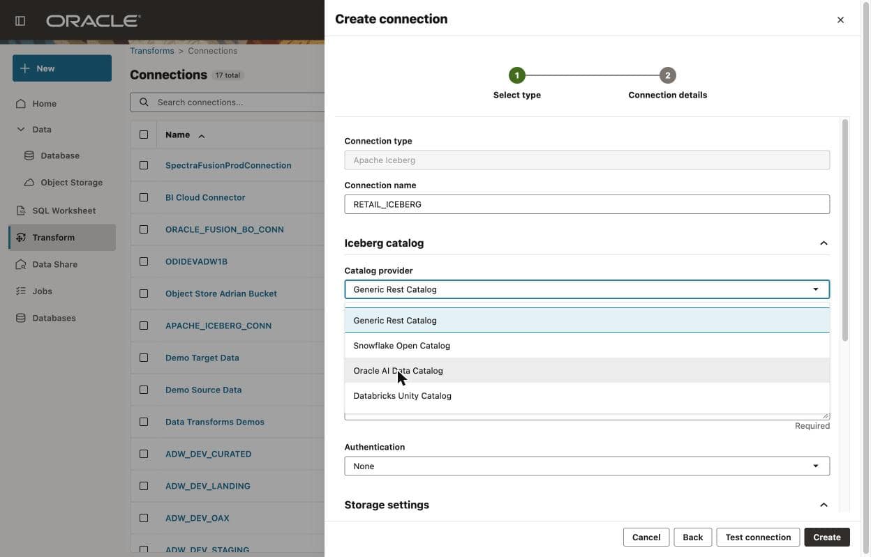
Figure 2. Choosing a catalog provider for an Apache Iceberg connection.
Why the catalog choice matters
The catalog is where an Iceberg table is discovered, governed and secured. Writing through it, rather than dropping files into a bucket, means the table appears with its permissions and lineage in place for whoever consumes it. For the retailer, ORDER_LINES lands once and appears in Unity Catalog for the data science team and in Autonomous AI Lakehouse for the analysts. If the consumer changes next year, you change the connection, not the pipeline.
2. Compaction and clustering: keeping tables healthy
Why Iceberg tables slow down
Iceberg never modifies a data file in place. Each commit writes new Parquet files and a new snapshot that points to them. That design gives Iceberg its time travel and safe concurrent reads, but it has a cost. A table loaded every 15 minutes gains roughly a hundred commits a day, each adding small files, and updates and deletes add more. Query engines then have to open many small files, manifests grow, and because every file contains a bit of every key range, the per-file minimum and maximum values that engines use to skip files stop being useful.
Compaction
Compaction rewrites many small files into fewer, larger ones and commits the result as a new snapshot. The data is the same; there is less of the overhead of opening, listing and tracking files, and the manifests shrink with it.
Clustering
Clustering goes further: it rewrites files so that rows with similar values in the clustering columns are stored together. Each file then covers a narrow range of, say, ORDER_DATE or CUSTOMER_ID, so a query with a filter on those columns can skip most files using only their metadata. Choose the columns that appear most often in filters and joins.
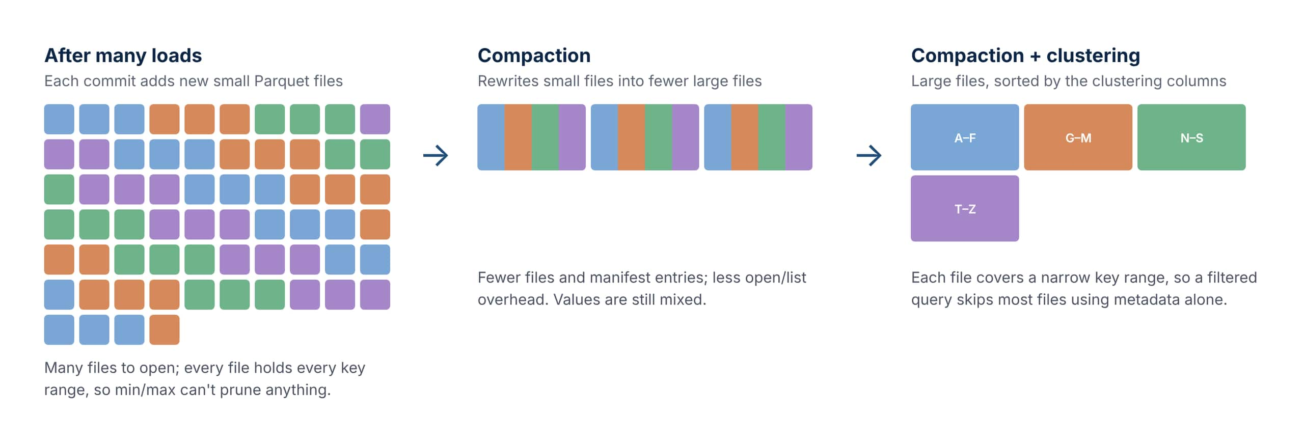
Figure 3. Compaction reduces the number of files; clustering makes each file cover a narrow range of values.
Maintenance as workflow steps
In Data Transforms, maintenance is not a separate system. You add it to a workflow next to the Iceberg data load, with five actions to choose from:
- Compaction of the table’s Parquet files.
- Clustering on the columns you choose.
- Compaction plus clustering in a single rewrite.
- Incremental compaction and incremental clustering, which focus on recently written data rather than rewriting the whole table, so they are cheap enough to run after frequent loads.
For the retailer, a sensible pattern is incremental compaction after each 15-minute load and a full compaction plus clustering on ORDER_DATE once a week. Because these are ordinary workflow steps, they inherit the scheduling, monitoring and failure handling of the workflow they belong to.
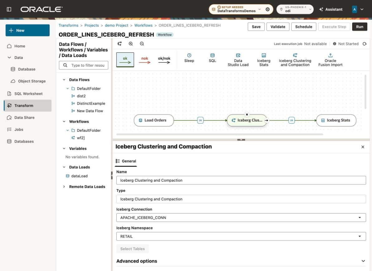
Figure 4. Load, maintain and refresh statistics in a single workflow.
3. Statistics from metadata, not scans
Why statistics matter
When Autonomous AI Lakehouse queries an Iceberg table, the optimizer needs to know how many rows the table has, how many are null in each column, the range of values and how many are distinct. Those numbers decide join order, join method, parallelism and whether a filter is selective. Without them the optimizer guesses, and on a large lakehouse table a wrong guess can turn a seconds-long query into a minutes-long one. And because a table like ORDER_LINES changes every 15 minutes, statistics go stale quickly.
The usual trade-off
The conventional way to gather statistics on an external table is to read its data, either all of it or a sample. That forces a choice:
- A small sample is fast but inaccurate. It misses the true minimum and maximum and rare values, and distinct counts extrapolated from a few percent of the rows are often badly wrong, especially on skewed data.
- A large sample or a full scan is accurate but expensive. It reads a large share of the table from object storage every time, which on a multi-terabyte table means long runtimes and real compute cost, repeated after every load.
In practice, many teams pick neither and live with stale statistics.
What Iceberg already knows
Iceberg removes the trade-off, because the statistics are already in the table’s metadata. When an engine writes a data file, it records the file in a manifest along with statistics computed from every row it wrote: the record count, and for each column the number of null values and the lower and upper bounds. The snapshot summary carries the table’s total record count. A simplified manifest entry looks like this:
{ "data_file": {

    "file_path": "s3://retail/order_lines/data/00017-4a1c.parquet",

    "record_count": 1843902,

    "null_value_counts": { "order_date": 0, "promo_code": 1210334 },

    "lower_bounds": { "order_date": "2026-10-01", "customer_id": 100045 },

    "upper_bounds": { "order_date": "2026-10-07", "customer_id": 994812 }

} }
The Iceberg Stats step in Data Transforms computes table and column statistics by aggregating this metadata, and then publishes them to the database so the optimizer can use them. It does not read the data files.
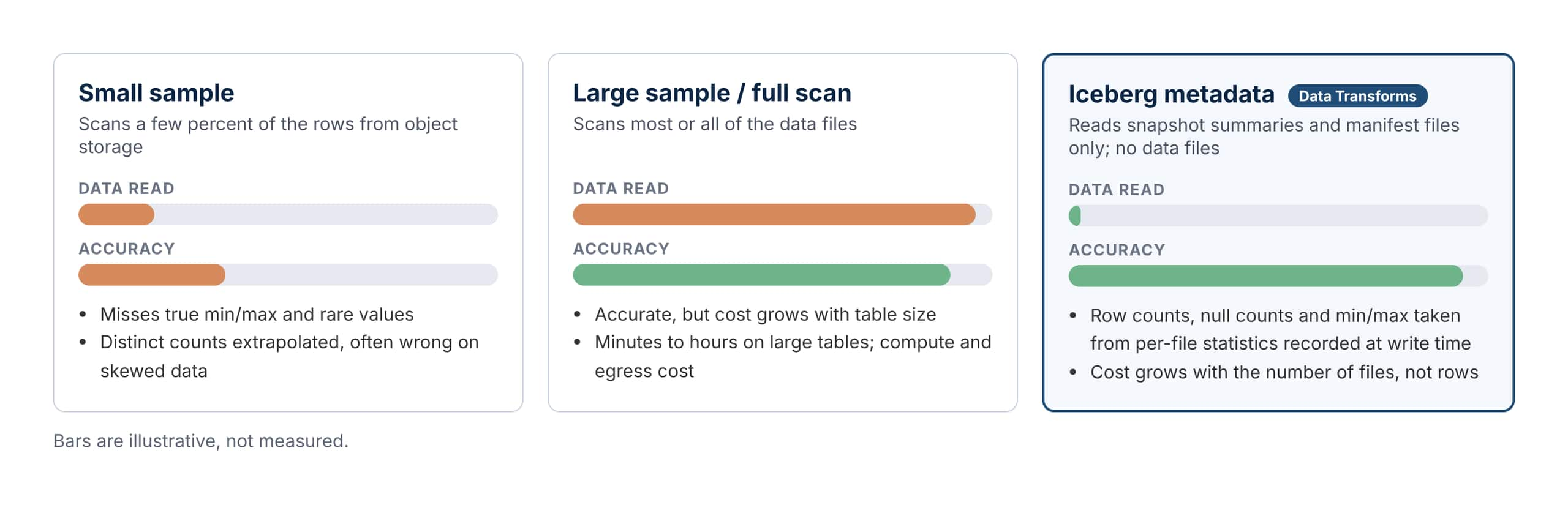
Figure 5. Three ways to get statistics for an Iceberg table.
Faster and more accurate
Statistics from metadata beat both sampling options at once:
- Faster than a large sample. The work is proportional to the number of files, not the number of rows. Manifests are a tiny fraction of the size of the data they describe, so refreshing statistics on a multi-terabyte table means reading metadata, not terabytes of Parquet from object storage. That makes it practical to refresh after every load.
- More accurate than a small sample. Row counts, null counts and minimum and maximum values are computed from every row when the file is written, so the aggregates are exact rather than estimated. Extremes and rare values that a sample misses are captured.
One detail worth knowing: Iceberg writers may truncate the bounds of long string columns to keep manifests small, so for those columns the recorded minimum and maximum are prefixes. Numeric, date and timestamp bounds are exact.
Using the Iceberg Stats step
Add the Iceberg Stats step to a workflow, select the Iceberg connection, then select the Oracle connection and the schema that holds the external tables over the Iceberg data. You can refresh statistics for selected tables or for all relevant external tables in the schema. Place it after the data load and any maintenance step, so the optimizer sees the table as it is after the latest commit.
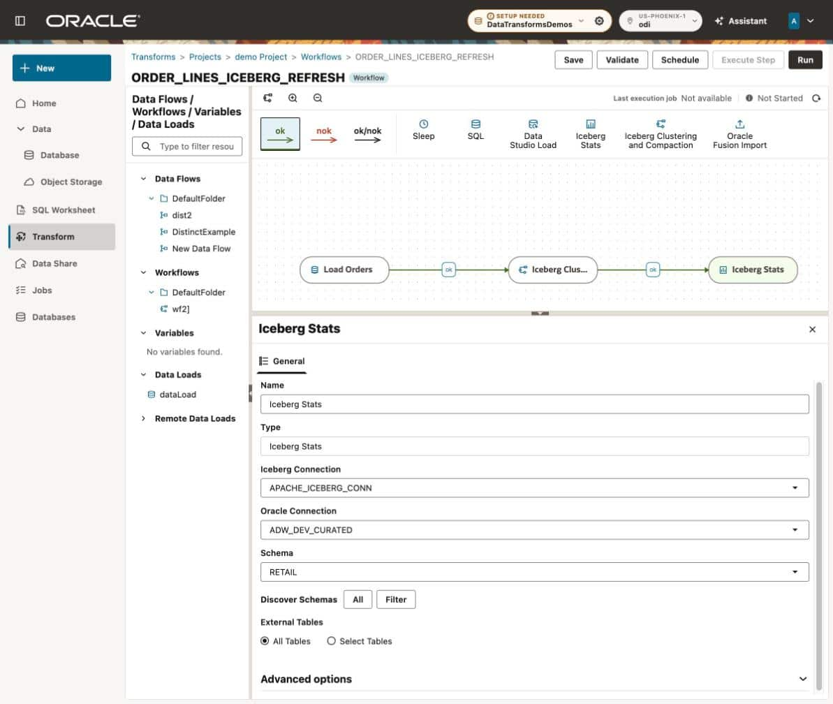
Figure 6. Configuring the Iceberg Stats step.
How the three reinforce each other
Compaction, clustering and statistics are each useful alone, and better together. Compaction reduces the number of manifest entries, so statistics are cheaper to compute. Clustering narrows the value range of each file, which makes file-level bounds much more informative for both file skipping and the optimizer. And fresh statistics let the optimizer take advantage of the layout that compaction and clustering produced. All three rely on the same idea: Iceberg’s metadata, kept in good shape, does most of the work.
4. Iceberg layers and the medallion architecture
Most lakehouse teams organize Iceberg tables in layers, usually called bronze, silver and gold: raw data lands in bronze, is cleaned and conformed into silver, and is aggregated into gold tables that analysts and applications consume. The catalog, maintenance and statistics capabilities above each matter at a different layer, and Data Transforms lets you build all three layers as one set of workflows.
Bronze: land it once, through the catalog. A Data Load writes the raw order lines from the order management system into an Iceberg table, ORDER_LINES_RAW, through the catalog your organization uses. Because the table is registered in the catalog as it is written, it is immediately governed and discoverable, and every downstream engine sees the same copy. Bronze tables take frequent, small appends, which is exactly the pattern that creates small files, so incremental compaction after each load belongs here.
Silver: clean, conform and cluster. Data flows read the bronze table through its external table in the Lakehouse and apply the rules that make the data trustworthy: deduplicate replayed records, standardize codes, resolve product and customer keys, and reject rows that fail validation into a quarantine table. The cleaned result is written to the Lakehouse, and a Data Load lands it in the catalog as the Iceberg table ORDER_LINES, the table the retailer’s analysts and data scientists share. Today the Data Load is the step that writes Iceberg; the data flow does the transformation work in the Lakehouse. Silver is where clustering pays off most: cluster on the columns people filter and join on, such as ORDER_DATE and CUSTOMER_ID, so both Autonomous AI Lakehouse and Databricks skip most files on a typical query.
Gold: aggregate for consumers. Gold tables such as DAILY_SALES_BY_CATEGORY or CUSTOMER_RETURN_RATE are built by data flows that join silver tables and aggregate them for a specific audience, then landed as Iceberg the same way. They are small compared with silver, read far more often, and change on a predictable schedule, so a full compaction plus clustering after each rebuild keeps them compact, and the Iceberg Stats step after that keeps the optimizer’s picture of them exact.
One workflow per layer, or one for all three. Each layer follows the same pattern in Data Transforms: load or transform, then maintain, then refresh statistics. With parallel workflows, independent bronze loads run side by side, silver flows start as soon as their bronze inputs finish, and gold rebuilds wait for the silver tables they depend on. The medallion layers become a dependency graph in one tool, with one schedule and one monitoring view, rather than a load tool, a Spark maintenance job and a database statistics job owned by three teams.
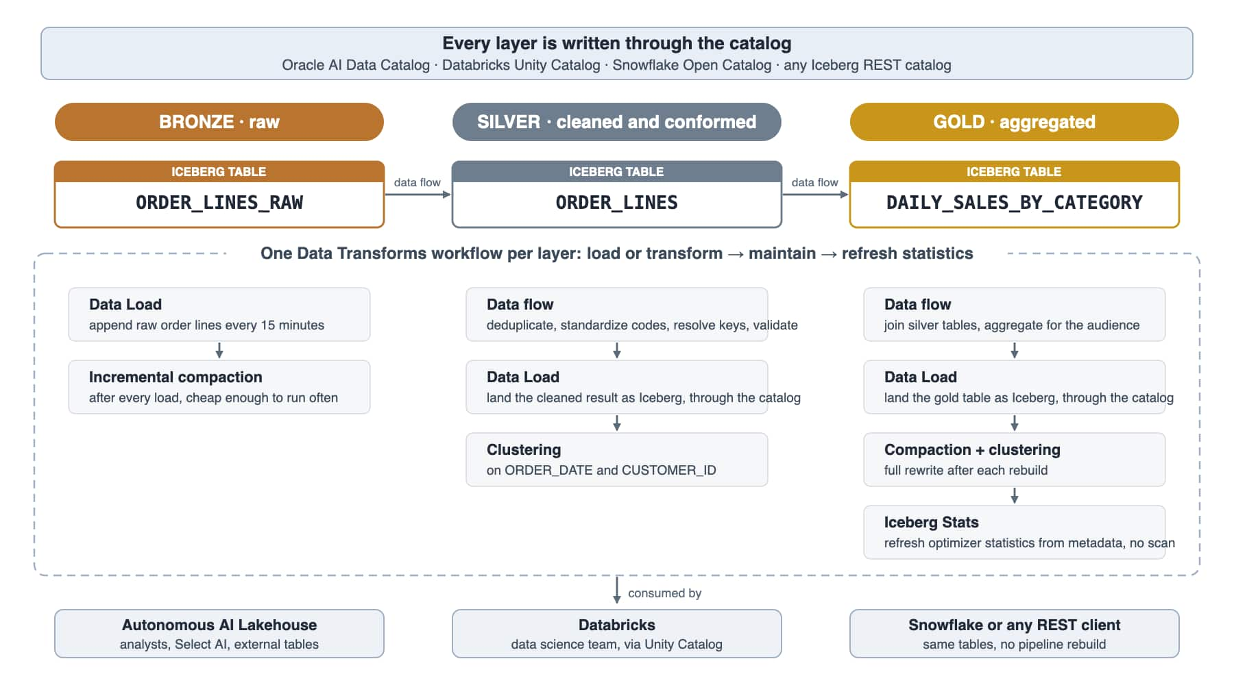
Figure 7. Bronze, silver and gold Iceberg tables, each with its load, maintenance and statistics steps in one Data Transforms workflow.
Why the catalog choice matters here. Because every layer is written through the catalog, the bronze and silver tables can serve engines you did not plan for. The data science team can read silver from Databricks today; if a new team adopts Snowflake next year, the same tables are reachable through Snowflake Open Catalog without rebuilding the pipelines.
Bringing it together
Data Transforms treats Iceberg as a first-class lakehouse target, not just another file format. One connector writes through Oracle AI Data Catalog, Databricks Unity Catalog, Snowflake Open Catalog or any Iceberg REST catalog, so data lands where it will be governed and consumed. Compaction and clustering keep the tables efficient as loads accumulate, and statistics computed from metadata keep the optimizer informed without the cost of scanning the data.
The practical advice is simple: build Iceberg pipelines as a single workflow of load, then compact or cluster, then refresh statistics. Maintenance and statistics then stay as current as the data, on the same schedule, with nothing extra to run.
Start building pipelines with Oracle Data Transforms at datastudio.oracle.com.