Introduction
In this post, we walk through how to efficiently load a massive volume of geospatial data, stored as Parquet files in an Oracle Cloud Infrastructure (OCI) Object Storage bucket, into a target table inside an Oracle Autonomous AI Database (ADB) deployed as Autonomous AI Lakehouse (ALH). We define external tables and populate internal tables leveraging ADB’s native support for external data formats, spatial types, and bulk data ingestion best practices.
By the end of this guide, you will know how to:
- Set up access to OCI Object Storage and map external tables to Parquet file groups.
- Create a target table using partitioning and interleaved clustering to optimize storage, and implement a spatial index to improve query efficiency on geospatial columns.
- Perform an initial direct-path bulk load on a target table that has no indexes yet.
- Optimize spatial data ingestion using an
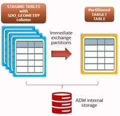
SDO_GEOMETRYcolumn. - Prepare and execute an efficient bulk load via the Exchange Partition technique. This approach is appropriate when the target table already has indexes (spatial or non-spatial) and we need to ingest very large datasets, as is typical for geospatial workloads.
The loading method described in this blog is valid for both small and very large datasets, including ingestion of tens of billions of rows.
The ingestion flow from Parquet files in OCI Object Storage to an Autonomous AI Lakehouse can be viewed as the LOAD phase of an ELT (Extract-Load-Transform) process required in a modern data warehousing project. The initial EXTRACT phase generates and positions the Parquet files from source systems. The final TRANSFORM phase runs immediately after the LOAD phase, directly inside ADB, taking advantage of its scalable compute and the business logic without adding extra architectural components.
Architectural model: ingestion from Parquet files to Autonomous AI Lakehouse
In this scenario we work with several billions of geospatial records stored as Parquet files in an OCI Object Storage bucket. These files contain several columns, including geometries (for example, points, lines, polygons). In our specific case we handle longitude and latitude coordinates.
The diagram below illustrates the steps explained in this post at a high level:
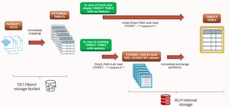
- Define external tables on the Parquet files. Using
DBMS_CLOUD.CREATE_EXTERNAL_TABLE, we map one or more external tables, each pointing to a group of Parquet files in the bucket.
From there the path depends on the state of the target table:
- If the target is a brand-new empty partitioned table with no indexes, the most performant strategy is a direct parallel direct-path bulk load (
INSERT /*+ APPEND PARALLEL(n) */) from the external table. Local indexes (spatial and non-spatial) are created afterwards. - If the target is an existing partitioned table that already has local indexes, a direct bulk insert is no longer the best choice because index maintenance during INSERT degrades throughput. The workaround is a two-phase approach: direct-path load into a staging table first (staging tables have no indexes, so the load is very fast), create the matching indexes on the staging table, then exchange partition with the target. The exchange is a metadata-only operation.
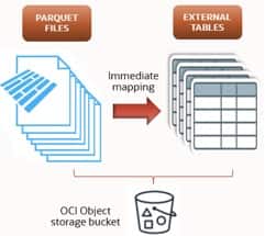
Mapping Parquet files with external tables
The goal of this first step is to map the Parquet files to one or more external tables, typically grouping a number of files per table.
Create the credential used to access the Object Storage bucket where the Parquet files reside. Follow the LiveLabs steps for the full procedure. Below is a credential template; we will use the name OBJS_CRED throughout this guide:
BEGIN
  DBMS_CLOUD.CREATE_CREDENTIAL (
    credential_name => 'OBJS_CRED',
    username        => '<tenancy_identity_domain>/<tenancy_account>',
    password        => '<authentication_token>'
  );
END;
/
ADB supports Parquet mapping not only from OCI Object Storage but also from any S3-compatible object store reachable via DBMS_CLOUD.
In the example below we map a single external table called EXT_TABLE_01 against n folders containing Parquet files, using the credential defined above. A more elaborate mapping (multiple external tables, finer-grained file groups) can be created based on project requirements. Creation is a metadata operation, so it completes in moments regardless of the number of underlying rows:
BEGIN
  DBMS_CLOUD.CREATE_EXTERNAL_TABLE(
    table_name      => 'EXT_TABLE_01',
    credential_name => 'OBJS_CRED',
    file_uri_list   =>
      'https://<namespace>.objectstorage.<region>.oraclecloud.com/n/<namespace>/b/<bucket>/o/FOLDER1/data_*.parquet,
       ...,
       https://<namespace>.objectstorage.<region>.oraclecloud.com/n/<namespace>/b/<bucket>/o/FOLDERn/data_*.parquet',
    format          => '{"type":"parquet", "schema":"first"}'
  );
END;
/
Where:
- The
formatparameter can be edited to match other supported file types — Parquet, CSV, Avro, ORC, JSON, gzip, and more — per the DBMS_CLOUD documentation. You can also apply specific data filters, for example to filter on different columns at read time.
Having the external mapping in place lets us inspect the Parquet table’s content, check column data types and row counts, and quickly re-map if needed.
Target table initial bulk load from external table
As described in the architectural overview above, when the target is an empty partitioned table with no indexes, the best approach is a direct-path load straight from the external table.
A target template table DDL:
CREATE TABLE TARGET_TABLE (
  RECORD_ID      VARCHAR2(4000),
  REQUEST_TIME   TIMESTAMP(3),
  ...
  GEO_LAT        NUMBER(38,15),
  GEO_LON        NUMBER(38,15),
  GEOM           SDO_GEOMETRY,
  ...
  FIELDn_1       VARCHAR2(32767),
  FIELDn         NUMBER(10)
)
CLUSTERING BY INTERLEAVED ORDER (request_time, geo_lon, geo_lat)
  YES ON LOAD YES ON DATA MOVEMENT
PARTITION BY RANGE (request_time) (
  PARTITION p20240501 VALUES LESS THAN (TIMESTAMP '2024-05-01 00:00:00')
    SEGMENT CREATION DEFERRED
);
Where:
- PARTITION BY RANGE (<partition_key_col>): this example uses a single target table partitioned by 1-hour time ranges, with the timestamp column as the partitioning key.
- Attribute clustering:
CLUSTERING BY INTERLEAVED ORDER (...) YES ON LOADensures that during massive ingestion rows are physically ordered by(request_time, geo_lon, geo_lat)at write time. This enables zone-map pruning on top of partition pruning and reduces I/O for subsequent time-range and geospatial queries, with no post-load reorganization cost. - The
GEO_LON/GEO_LATNUMBER columns are required for the clustering clause. TheGEOM SDO_GEOMETRYcolumn is added for spatial-index creation and spatial query performance.
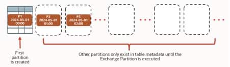
The PL/SQL block below pre-creates a number of partitions of one hour each, covering a fixed period of n days (n × 24 partitions). Pre-creating partitions is required by the Exchange Partition method, which needs the empty target partitions to already exist.
Alternatively we could add an INTERVAL (NUMTODSINTERVAL(1, 'HOUR')) clause to have partitions created on the fly during the load — useful when ingesting via direct-path INSERT directly into the target. In our template, the first partition p20240501 catches all data prior to the specified date.
DECLARE
  part_num NUMBER       := 2;
  t        TIMESTAMP(3) := TIMESTAMP '2024-05-01 00:00:00';
BEGIN
  FOR r IN 1 .. n*24 LOOP   -- n is the number of days the partitions should cover
    t := t + INTERVAL '1' HOUR;
    EXECUTE IMMEDIATE
      'ALTER TABLE TARGET_TABLE ADD PARTITION p' || part_num ||
      ' VALUES LESS THAN (TIMESTAMP ''' ||
      TO_CHAR(CAST(t AS DATE), 'YYYY-MM-DD HH24:MI:SS') || ''')';
    part_num := part_num + 1;
  END LOOP;
END;
/
For optimal performance the initial bulk load into the target table should be done before any indexes exist:
ALTER SESSION SET optimizer_ignore_hints          = FALSE;
ALTER SESSION SET optimizer_ignore_parallel_hints = FALSE;
ALTER SESSION ENABLE PARALLEL DML;
ALTER SESSION ENABLE PARALLEL QUERY;

INSERT /*+ APPEND PARALLEL(tg_table, n) */
INTO TARGET_TABLE tg_table NOLOGGING
SELECT
  RECORD_ID,
  REQUEST_TIME,
  ...
  GEO_LAT,
  GEO_LON,
  SDO_GEOMETRY(2001, 4326, SDO_POINT_TYPE(GEO_LON, GEO_LAT, NULL), NULL, NULL),
  ...
  FIELDn_1,
  FIELDn
FROM EXT_TABLE_01;
COMMIT;
In Autonomous AI Lakehouse, both optimizer_ignore_hints and optimizer_ignore_parallel_hints default to TRUE (hints are ignored, to protect the workload). For a deliberate, one-off direct-path load we explicitly set them to FALSE at the session level so APPEND and PARALLEL(n) are honored.
Once the target table has indexes, subsequent very large bulk loads should use the Exchange Partition method described below to avoid index-maintenance overhead. Subsequent smaller loads can still use direct-path INSERT straight into the target.
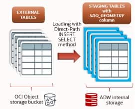
Loading from external table to staging table
When the target table already has indexes, we use the staging-table pattern for a fast load, and then move the data via Exchange Partition.
The staging-table structure can be derived from the external table, but in our scenario we add a GEOM column of type SDO_GEOMETRY, so we recreate the table manually. Depending on requirements you may use a 1:1, 1:n, n:1, or n:n mapping between external and staging tables.
CREATE TABLE STAGE_TABLE_01 (
  RECORD_ID      VARCHAR2(4000),
  REQUEST_TIME   TIMESTAMP(3),
  ...
  GEO_LAT        NUMBER(38,6),
  GEO_LON        NUMBER(38,6),
  GEOM           SDO_GEOMETRY,
  ...
  FIELDn_1       VARCHAR2(32767),
  FIELDn         NUMBER(10)
)
FOR STAGING
CLUSTERING BY INTERLEAVED ORDER (request_time, geo_lon, geo_lat)
  YES ON LOAD YES ON DATA MOVEMENT;
Where:
- CLUSTERING BY INTERLEAVED ORDER (<col1>, <col2>, …): physically co-locates and sorts data on disk by the listed columns — here, the timestamp partition key and the spatial coordinates. The database can then skip blocks that don’t match time/location predicates. This clause must match the target table so that the Exchange Partition succeeds.
- SDO_GEOMETRY is provided by Oracle Spatial. It stores and manipulates geospatial data (points, lines, polygons) and is the data type that lets us run queries with the built-in spatial functions.
- FOR STAGING: enables a table optimized for loading data into a lakehouse (compression disabled, dynamic sampling). See the ADB-Serverless data warehouse workload documentation for details.
Template for loading data from the external table into a staging table using direct-path INSERT:
ALTER SESSION SET optimizer_ignore_hints          = FALSE;
ALTER SESSION SET optimizer_ignore_parallel_hints = FALSE;
ALTER SESSION ENABLE PARALLEL DML;
ALTER SESSION ENABLE PARALLEL QUERY;

INSERT /*+ APPEND PARALLEL(stg01, n) */
INTO STAGE_TABLE_01 stg01 NOLOGGING
SELECT
  RECORD_ID,
  REQUEST_TIME,
  ...
  GEO_LAT,
  GEO_LON,
  SDO_GEOMETRY(2001, 4326, SDO_POINT_TYPE(GEO_LON, GEO_LAT, NULL), NULL, NULL),
  ...
  FIELDn_1,
  FIELDn
FROM EXT_TABLE_01
WHERE REQUEST_TIME >= TIMESTAMP '2024-05-15 00:00:00'
  AND REQUEST_TIME <  TIMESTAMP '2024-05-15 01:00:00';   -- one hour window
COMMIT;
The SDO_GEOMETRY constructor used above means:
2001: geometry type — a 2D point.4326: SRID for WGS 84, the standard GPS coordinate system.SDO_POINT_TYPE(GEO_LON, GEO_LAT, NULL): the (X, Y, Z) values of the point — longitude (X), latitude (Y), no Z (no elevation).- The trailing two NULLs mean
SDO_ELEM_INFOandSDO_ORDINATESare not needed for a simple point.
Other clauses worth calling out:
/*+ APPEND PARALLEL(table_alias, n) */: direct-path insert in parallel, with degreenscaled to the ECPU allocation (for example 16).NOLOGGING: minimizes redo generation, faster load.WHEREclause: filters one hour of data, i.e. the window that maps exactly to one target partition. Each staging table corresponds to one target partition, which is the prerequisite for Exchange Partition. Adjust the window to your partition size.
Preparing the staging and target tables for the Exchange Partition
At this point the staging tables hold data that maps 1:1 to a single target partition each. Now we prepare the target and staging table structures for the final step — moving the data into the target partitions via Exchange Partition.
Exchange Partition requires that the indexes on the two tables match.
The target table will typically have a spatial index on GEOM plus other non-spatial B-tree indexes. We create matching indexes on both tables: LOCAL on the target (because it is partitioned), GLOBAL on the staging table.
Spatial index on the GEOM column. First, register the spatial metadata for the staging table:
INSERT INTO user_sdo_geom_metadata VALUES (
  'STAGE_TABLE_01', 'GEOM',
  SDO_DIM_ARRAY(
    SDO_DIM_ELEMENT('x', -180, 180, .005),
    SDO_DIM_ELEMENT('y',  -90,  90, .005)
  ),
  4326
);
- Before creating the spatial index, insert a row into
user_sdo_geom_metadata. SDO_DIM_ARRAY(...)defines the dimensional boundaries — the valid range and tolerance for the coordinates in your data.
Then create the spatial index on the staging table:
CREATE INDEX SIDX_STAGE_TABLE_GEOM ON STAGE_TABLE_01 (GEOM)
  INDEXTYPE IS mdsys.spatial_index_v2
  PARAMETERS ('layer_gtype=point cbtree_index=true sdo_point_field_only=true')
  PARALLEL n;   -- adjust based on ECPU allocation (e.g. 16)
Per the Exchange Partition requirements, also create any non-spatial indexes on the staging table that exist on the target.
Spatial index creation on the target table
Adding a spatial index to a table with an SDO_GEOMETRY column improves spatial-query performance significantly. With a spatial index you can:
- Quickly locate geometries based on spatial relationships (within, intersects, near).
- Avoid full table scans for spatial predicates.
- Accelerate spatial joins using operators such as
SDO_ANYINTERACT,SDO_WITHIN_DISTANCE, etc.
Without a spatial index, the database would scan the entire table to find rows in a given geographic region — impractical for large datasets such as billions of point coordinates.
Register the spatial metadata for the target table:
INSERT INTO user_sdo_geom_metadata VALUES (
  'TARGET_TABLE', 'GEOM',
  SDO_DIM_ARRAY(
    SDO_DIM_ELEMENT('x', -180, 180, .005),
    SDO_DIM_ELEMENT('y',  -90,  90, .005)
  ),
  4326
);
Building the index from scratch after the data is loaded is typically much faster than maintaining it during the load. A common pattern in Oracle is to create the index UNUSABLE first and rebuild partition by partition — this lets you verify each index partition incrementally.
CREATE INDEX SIDX_TARGET_TABLE_GEOM ON TARGET_TABLE (GEOM)
  INDEXTYPE IS mdsys.spatial_index_v2
  PARAMETERS ('layer_gtype=point cbtree_index=true sdo_point_field_only=true')
  PARALLEL n   -- adjust based on ECPU allocation (e.g. 16)
  LOCAL UNUSABLE;
The LOCAL clause creates a separate spatial index segment for each partition, which is essential for managing large partitioned tables efficiently.
Procedure to rebuild the partitioned index — one partition at a time, optimizing the index for the latest data and verifying integrity as we go:
DECLARE
  table_name_v   VARCHAR2(100) := 'TARGET_TABLE';
  index_name_v   VARCHAR2(100) := 'SIDX_TARGET_TABLE_GEOM';
  parallel_deg_v NUMBER        := 16;   -- adjust to available resources
BEGIN
  FOR r IN (
    SELECT partition_name
    FROM   user_tab_partitions
    WHERE  table_name = table_name_v
    AND    segment_created = 'YES'
    ORDER  BY 1
  ) LOOP
    EXECUTE IMMEDIATE
      'ALTER INDEX ' || index_name_v ||
      ' REBUILD PARTITION ' || r.partition_name ||
      ' PARALLEL ' || parallel_deg_v;
  END LOOP;
END;
/
Where:
segment_created = 'YES': rebuilds only partitions that have a materialized segment (i.e. contain data).parallel_deg_vis optional; set it to match the resources available, to speed up the rebuild.
Spatial index parameter notes:
- spatial_index_v2: the current recommended spatial index type — supersedes the older
spatial_index. - layer_gtype=point: tells the index that the data is point geometry; highly optimized for point data versus more complex polygons or lines.
- cbtree_index=true: CBTREE spatial indexes are a point-only spatial index, optimized for spatial searches and DML on point data, especially concurrent DML over multiple connections (for example via a connection pool).
- sdo_point_field_only=true: a critical optimization for tables that contain only point data with all points stored in the
sdo_pointattribute of thesdo_geometryobject. Speeds up both index creation and query execution.
Once you run queries against the table, check the execution plan to confirm the spatial index is being used.
Loading the target table with the Exchange Partition technique
With the target ready and each staging table holding only the rows that belong to a specific partition time window, the Exchange Partition command moves the data into the matching empty target partition almost instantly. Oracle swaps the segment metadata between the staging table and the target partition rather than physically copying rows, so the operation is extremely fast even for very large datasets.
Exchange Partition completes in milliseconds and avoids the index-maintenance overhead that would otherwise apply to large INSERTs on an indexed target.
For smaller ingests, direct-path INSERT straight into the partitioned target — while indexes are maintained — remains a reliable alternative. The use case here justifies Exchange Partition because we are ingesting millions of rows per hour into the target table.
Example applied to a single partition:
ALTER TABLE TARGET_TABLE
  EXCHANGE PARTITION p_20240501_00
  WITH TABLE STAGE_TABLE_01
  INCLUDING INDEXES
  WITHOUT VALIDATION;
INCLUDING INDEXES ensures that local indexes are exchanged together with the segment. Combined with WITHOUT VALIDATION and a properly defined CHECK constraint on the staging table that matches the target partition boundaries, you avoid any row-by-row verification. The result is a near-instant, zero-downtime load of partitioned data.
Assuming all the staging tables are ready, this operation is easy to automate with a loop across the necessary partitions.
Conclusion
In this post we walked through the end-to-end process of ingesting geospatial data stored as Parquet files in OCI Object Storage into a partitioned table inside Oracle Autonomous AI Lakehouse (ALH). Using ALH’s native support for Parquet and its spatial-data capabilities, we built a cloud-native workflow that handles location-based data in a modern ELT pipeline — using direct-path bulk load for the empty-target case and Exchange Partition for the indexed-target case.
With features such as the DBMS_CLOUD package, external tables, attribute clustering and spatial indexing, ALH lets you work with large-scale geospatial datasets using familiar SQL. Partitioning enhances query performance and data organization, especially with time-series or regionally segmented data. This workflow simplifies data ingestion and enables spatial analytics and real-time reporting inside a secure, autonomous, scalable cloud database platform.