
Hybrid retrieval for agent memory combines semantic candidates, lexical matches, and explicit scope before assembling context. Fusion and reranking are useful only when they improve a labeled workload without admitting stale or unauthorized memory.
Hybrid retrieval for agent memory is a multi-stage pipeline. Pure vector search is the prototype.
The companion repo implements the full pipeline against the schema and two-layer pattern from Persistent Memory and Derived Context, From Prompt to Persistence part 1, and part 2: hybrid SQL with in-database PREDICTION reranking, a LangChain retriever, a LangGraph retrieval graph, and the evaluation suite with its golden-set labeling flow, runnable end to end against an Oracle AI Database 26ai Free instance on the 23-document research corpus built for this article.
Companion notebook: Hybrid Retrieval Pipeline
Key takeaways
- Hybrid retrieval for agent memory starts with database-enforced metadata filters. It then combines vector and lexical candidates through rank fusion, with optional reranking.
- Vector search finds semantic matches. Lexical search pins identifiers and exact strings. SQL and JSON metadata constrain scope and lifecycle before applying source and type restrictions. Those filters run before either search mode ranks a row.
- Every stage has to earn its place on a labeled set. In the companion experiment, equal-weight hybrid fusion underperformed vector search on the small corpus, while reranking improved ordering at a material latency cost.
Jane’s research assistant at Acme has good days and bad days. Some answers are sharp, cited, exactly right. Others are vaguely on-topic in a way that’s hard to complain about but impossible to trust. There’s no obvious pattern. Same model, same prompt template, same memory schema underneath. The team suspects the model, because the model is the part everyone watches.
Retrieval is often the first place to look. When the right rows reach the context window, the model has a better chance of producing a grounded answer. When they do not, even a capable model may answer confidently from the wrong material. The model cannot recover a passage the retrieval pipeline never supplied.
This is the third piece in a series. From Prompt to Persistence part 1 and part 2 built the multi-tenant schema: eight typed memory tables, four scope columns, row-level security on the tenant boundary, and provenance on every durable row. Persistent Memory and Derived Context separated the canonical layer from the derived layer so every retrieved row still points to something true.
Part 2 ended with vector and lexical scores side by side, deliberately unfused. This article picks up there. The schema stores the memory. The two-layer pattern keeps it honest. This pipeline reads it and assembles the working set the agent uses.
Why your agent feels slightly off
The question we’ll use throughout comes from the research assistant scenario the whole series has been building. Jane asks:
“What did the Letta paper say about memory eviction, and how does that compare to what the AgentCore docs recommend?”
This one sentence stresses every part of a retrieval system:
- “Letta” and “AgentCore” are exact-match identifiers. Embedding models under-weight rare proper nouns, so vector search will happily return chunks about memory management from papers that never mention either name.
- “Memory eviction” is a concept. The Letta paper might call it context pruning, message eviction, or recursive summarization. Lexical search will miss every paraphrase.
- “The docs the user has access to” is a scope constraint. Only ingested papers and vendor docs in collections Jane’s agent is allowed to read, inside Acme’s tenant boundary, should be candidates at all. No similarity score enforces that. Only a filter does.
- Comparing two sources means the context window needs good chunks from both documents rather than five redundant chunks from whichever one embeds closer to the query.
Run it through pure vector top-k against the research corpus the companion notebook builds and the answer surfaces AgentCore only incidentally, never the passage that answers the question. Run it through hybrid retrieval and both sources appear, with the first AgentCore retention passage at fused rank eleven. Reranking brings that passage to rank five, after four Letta passages. Context budgeting then preserves coverage from both sources so the agent can make the comparison Jane asked for.
Same model every time. The thing that moved was retrieval. That’s the thesis: retrieval is an architecture.
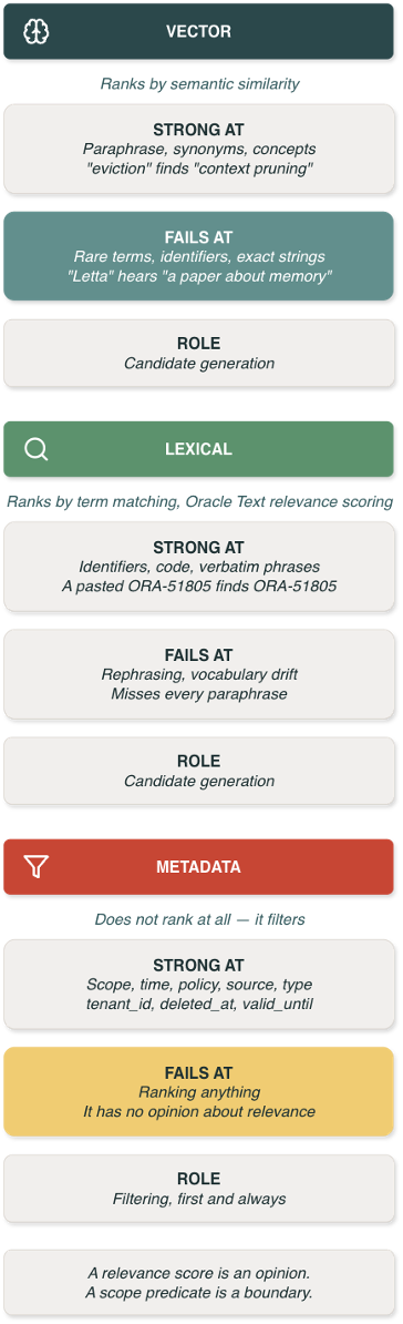
Vector, lexical, metadata: three retrieval modes, three failure modes
This pipeline uses three retrieval modes, and each one covers a failure mode the other two leave exposed. Whether both ranking modes earn a place depends on the corpus and query mix.
Vector retrieval ranks by semantic similarity. It’s the mode that handles paraphrase, synonyms, conceptual matches, the reason memory eviction can find a chunk about “pruning stale messages from the context window.” Its failure mode is specificity. Rare tokens, product names, error strings, version numbers, benchmark identifiers: all of them get diluted into an embedding that mostly encodes the surrounding topic. Ask a vector index about “Letta” and it hears “a paper about agent memory,” which describes half the corpus.
Lexical retrieval ranks by term matching using Oracle Text relevance scores. It’s the mode that nails exact identifiers, code fragments, error messages typed verbatim. A user who pastes ORA-51805 into the chat deserves the document containing ORA-51805, and no embedding model should be trusted with that job. Its failure mode is the inverse: any vocabulary shift between the query and the document breaks it. “Memory eviction” finds nothing in a paper that only ever says “context pruning.”
Metadata retrieval does not rank. It filters on scope, lifecycle, time, source, collection, and type. Those predicates become a security boundary only when the database enforces them with row-level security or an equivalent policy. An application filter is useful for retrieval scope, but it is not sufficient tenant isolation because a caller can forget it. A relevance score is an opinion. A database-enforced scope predicate is a boundary.
| Mode | Strong at | Fails at | Role in the pipeline |
| Vector | Paraphrase, synonyms, concepts | Rare terms, identifiers, exact strings | Candidate generation |
| Lexical | Identifiers, code, verbatim phrases | Rephrasing, vocabulary drift | Candidate generation |
| Metadata | Scope, time, policy, source, type | Ranking anything | Filtering; security when policy-enforced |
Jane’s question needs all three at once: metadata to bound the search to her tenant and collections, lexical to pin “Letta” and “AgentCore,” vector to find eviction discussed in other words. Only the filter is mandatory for correctness — a missing scope predicate is a security bug, while a missing retriever is only a quality one.
The hybrid retrieval pipeline, stage by stage
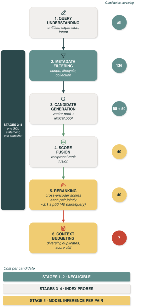
The order of stages follows one principle borrowed directly from query optimization: filter early, rerank late. Cheap, high-selectivity operations run first and shrink the candidate set. Expensive, high-precision operations run last, on the smallest set that still contains the answer. Databases have applied this thinking to query plans for fifty years. Retrieval pipelines are query plans, and most of them are written by people who’ve never looked at one.
Stage 1: query understanding. Before anything touches an index, the raw question gets decomposed: extract entities (“Letta”, “AgentCore”), expand the concept vocabulary (memory eviction to context pruning, message eviction, summarization), and classify intent. A factual lookup, a procedural recall, and an open-ended comparison want different candidate mixes from different tables. A production implementation can use one fast-model call that returns a small JSON object with entities and expanded terms, plus intent and time bounds. The companion notebook uses fixed rules and a small thesaurus for the same step. This keeps the demo repeatable and removes model-response variance from the retrieval comparison. The plan must still yield a valid lexical expression when a question has no proper nouns or thesaurus hits; the fallback is the question’s own content words.
Stage 2: metadata filtering. Apply scope and policy before any ranking happens. In the schema from From Prompt to Persistence (Part 1), the tenant predicate is appended by row-level security, so it’s enforced even if every other stage of the pipeline has a bug. The remaining predicates are the working scope block from part 1 (user_id/agent_id/thread_id with NULL inheritance, deleted_at IS NULL, valid_until still open) plus whatever the query understanding stage produced: collection restrictions, time windows, source types. This stage is typically cheaper than ranking and can shrink the candidate set substantially when the predicates are selective. Every row it removes is a row the expensive stages never touch.
Stage 3: hybrid candidate generation. Vector search and lexical search run against the filtered set, each producing its own ranked top-k (50 is a reasonable default for each side). They disagree with each other constantly, and that’s the point. The vector pool has the paraphrases. The lexical pool has the identifiers. The answer to Jane’s question lives in the union.
Stage 4: score fusion. Vector distances and lexical scores live on incompatible scales, so don’t combine the scores. Combine the ranks. Reciprocal rank fusion (RRF) gives each candidate 1/(60 + rank) from each list it appears in and sums them. RRF avoids score calibration and has one constant, conventionally set to 60. A calibrated linear combination can outperform it when measured score distributions support the added complexity, so treat RRF as a strong baseline rather than a guaranteed winner.
Stage 5: reranking. A cross-encoder scores the query and candidate together, which can improve ordering after candidate generation. It is also the most expensive stage, so it runs on 40 candidates instead of the full corpus. In the companion evaluation, this stage produced the largest NDCG gain, along with roughly 2.2 seconds of p50 added latency.
Stage 6: context budgeting. The token budget is fixed before retrieval starts, and the reranked list gets cut to fit it. The notebook uses a greedy budget pass instead of simple truncation: prefer diversity across source documents for a comparison question, drop near-duplicate chunks even when they score well, and stop early when scores fall off a cliff. More tokens of bad context is just more expensive bad context, and evaluations of long-context models show that task performance can drop when relevant material appears in the middle, exactly where a lazy pipeline dumps its marginal hits. What you didn’t include is a decision too. The output of this stage is the working set: the ranked, budgeted, provenance-tagged slice of memory that the agent loop’s Infer & Act phase actually consumes. How that working set gets ordered and laid out inside the prompt is the next article in this series; this pipeline’s job ends at deciding what earned a seat.
One thing worth making explicit, because it connects this article to the last one: the pipeline reads the derived layer, and only the derived layer, for ranking. Embeddings, text indexes, materialized projections: all of it is derived context, rebuilt from canonical memory under the sync policies from the two-layer article. The metadata filters run against canonical scope and lifecycle columns. Every candidate that survives to the working set carries its provenance (source_event_id, document ID, version) back to a canonical row. Fast path for ranking with true path for citation. The arrow between them points one direction.
The hybrid query in one SQL statement
Now the centerpiece. Stages 2 through 5 (metadata filtering, both candidate generators, RRF fusion, and the cross-encoder rescore) as one SQL statement against the knowledge base tables from part 1. Not an integration project. A query.
One piece of DDL is needed on top of the part 1 schema. Entity and summarization memory already carry Oracle Text indexes for their lexical halves; the knowledge base chunks need the same:
CREATE INDEX idx_kb_chunk_text ON knowledge_base_chunk (content)
  INDEXTYPE IS CTXSYS.CONTEXT PARAMETERS ('SYNC (ON COMMIT)');
With that in place, here’s Jane’s question as a query plan. :query is the natural-language question; :lex_query is the Oracle Text expression the query understanding stage built from the extracted entities and expanded terms (something like {Letta} OR {AgentCore} OR {memory eviction} OR {context pruning}. Brace every term. Oracle Text reserves ABOUT, ACCUM, AND, NEAR, NOT and WITHIN as operators, so an ordinary English word lifted from a user’s question is a syntax error unescaped. The question “where do models attend least within a long context?” fails on within. Braces make the content literal, which also handles hyphens, and it saves maintaining a reserved-word list that has to track Oracle’s):
WITH
-- Stage 3a: vector candidates over the metadata-filtered set
vec_pool AS (
  SELECT c.id,
         ROW_NUMBER() OVER (
           ORDER BY VECTOR_DISTANCE(c.embedding,
             VECTOR_EMBEDDING(ALL_MINILM_L12_V2 USING :query AS DATA),
             COSINE)) AS vec_rank
    FROM knowledge_base_chunk c
    JOIN knowledge_base_document d ON d.id = c.document_id
   WHERE d.collection IN ('ingested-papers', 'vendor-docs')     -- Stage 2 starts here
     AND d.valid_until IS NULL AND d.deleted_at IS NULL
     AND c.deleted_at IS NULL
     AND (d.user_id IS NULL OR d.user_id = :user_id)
     AND JSON_VALUE(c.metadata, '$.section_type') <> 'references'
   ORDER BY VECTOR_DISTANCE(c.embedding,
             VECTOR_EMBEDDING(ALL_MINILM_L12_V2 USING :query AS DATA),
             COSINE)
   FETCH FIRST 50 ROWS ONLY
),
-- Stage 3b: lexical candidates over the same filtered set
lex_pool AS (
  SELECT c.id,
         DENSE_RANK() OVER (ORDER BY SCORE(1) DESC) AS lex_rank
    FROM knowledge_base_chunk c
    JOIN knowledge_base_document d ON d.id = c.document_id
   WHERE CONTAINS(c.content, :lex_query, 1) > 0
     AND d.collection IN ('ingested-papers', 'vendor-docs')
     AND d.valid_until IS NULL AND d.deleted_at IS NULL
     AND c.deleted_at IS NULL
     AND (d.user_id IS NULL OR d.user_id = :user_id)
     AND JSON_VALUE(c.metadata, '$.section_type') <> 'references'
   ORDER BY SCORE(1) DESC
   FETCH FIRST 50 ROWS ONLY
),
-- Stage 4: reciprocal rank fusion across the two pools
fused AS (
  SELECT COALESCE(v.id, l.id) AS id,
         COALESCE(1 / (60 + v.vec_rank), 0)
       + COALESCE(1 / (60 + l.lex_rank), 0) AS rrf_score
    FROM vec_pool v
    FULL OUTER JOIN lex_pool l ON v.id = l.id
),
candidates AS (
  SELECT id, rrf_score
    FROM fused
   ORDER BY rrf_score DESC
   FETCH FIRST 40 ROWS ONLY
)
SELECT c.id, c.content, c.chunk_index, c.metadata,
       d.id AS document_id, d.title, d.source_uri, d.version,
       k.rrf_score,
       PREDICTION(BGE_RERANKER USING :query AS FIRST_INPUT,
                  d.title || '. ' || c.content AS SECOND_INPUT) AS rerank_score
  FROM candidates k
  JOIN knowledge_base_chunk c    ON c.id = k.id
  JOIN knowledge_base_document d ON d.id = c.document_id
 ORDER BY rerank_score DESC;
-- tenant_id predicate appended automatically by RLS on every table reference
Walking the clauses:
- This example demonstrates the inherited
user_idscope predicate inside each pool. The tenant predicate does not appear because it cannot be forgotten: RLS appends it to every table reference, in both pools and on the final join, every time. Apply correspondingagent_idorthread_idpredicates when knowledge-base documents use those scopes; this shared research corpus is tenant- and user-scoped. That holds only if the policy loop from part 1 matchesKNOWLEDGE_BASE%as well as%_MEMORY. Both knowledge-base tables carrytenant_idbut neither name ends in_MEMORY, so an obvious loop leaves precisely the two tables this query reads without a policy, and the query has no predicate of its own to fall back on. JSON_VALUE(c.metadata, '$.section_type')is a derived-metadata filter, here excluding bibliography chunks that match “Letta” forty times without saying anything. Part 1’s functional index pattern on JSON paths makes this predicate indexable rather than a per-row parse.VECTOR_DISTANCEwith an in-databaseVECTOR_EMBEDDINGmeans the query text is embedded by the engine in the statement itself, with the HNSW (Hierarchical Navigable Small World) index from part 1 (ORGANIZATION INMEMORY NEIGHBOR GRAPH) available to the optimizer. On this 137-chunk run, Oracle chose a different physical plan.CONTAINS ... SCORE(1)is the Oracle Text half, running against the index we just created. Note that both pools repeat the same metadata predicates: each generator ranks only what the filters allow, which is what filter early means in practice. Note also that the lexical pool ranks withDENSE_RANKrather thanROW_NUMBER. Oracle TextSCORE()is a coarse integer, and on short chunks ties are the norm rather than the exception: one query against the companion notebook’s corpus matched 80 chunks across ten distinct scores.ROW_NUMBERwould order those tied chunks arbitrarily, and the next stage would read that arbitrary order as signal. This is the sharp edge on rank fusion generally: discarding the scores and trusting the order is what makes RRF insensitive to score scaling, and equally what makes it credulous when the order is partly noise.- The
FULL OUTER JOINplusCOALESCEarithmetic is RRF, in four lines. A chunk found by both generators gets both reciprocal terms and rises; a chunk found by only one still competes. This is the fusion that part 2’s query deferred: where that statement returnedvec_scoreandlex_scoreside by side and left the ranking to a later stage, this is the later stage. - The
candidatesCTE caps the set at 40 rows before reranking, which is Stage 5’s input contract.
The CTEs describe the logical stages. The optimizer still chooses the physical plan. In the companion run, the 137-chunk corpus was small enough that Oracle used the collection and chunk indexes, window sorts, and a full outer hash join without an HNSW step. A larger corpus may produce a different plan. Read the plan Oracle chose before tuning the plan you expected.
The plan below is condensed from the companion notebook’s DBMS_XPLAN output:
SORT ORDER BY STOPKEY
 NESTED LOOPS
  HASH JOIN FULL OUTER (RRF fusion)
   WINDOW SORT PUSHED RANK (vector pool)
    INDEX RANGE SCAN IDX_KB_DOC_COLLECTION
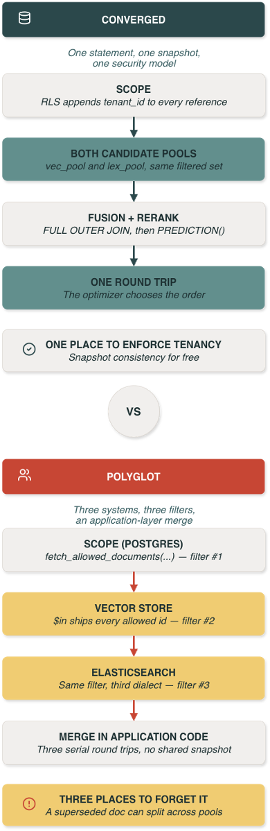
And one property that’s easy to miss because nothing visibly does it: the whole statement reads one transactional snapshot. The vector pool, the lexical pool, the final join: all of them see the same instant of the database. If a document is being superseded mid-query by a Promote step on another connection, this query sees it entirely old or entirely new, never a chunk from each. After the two-layer article made the case for keeping canonical and derived in sync, this is the read-side payoff: consistency you don’t write code for.
The polyglot version, for contrast
The same pipeline with a dedicated vector store, Elasticsearch for lexical, and Postgres for scope looks like this:
# 1. Resolve scope: which document IDs may this user see? (Postgres)
doc_ids = pg.fetch_allowed_documents(tenant_id, user_id,
                                 collections=['ingested-papers', 'vendor-docs'])

# 2. Vector candidates (vector store), filtered to allowed docs
vec_hits = vector_store.query(vector=embed(query), top_k=50,
                              filter={'tenant_id': tenant_id,
                                      'document_id': {'$in': doc_ids}})

# 3. Lexical candidates (Elasticsearch), same filter re-expressed in its DSL
lex_hits = es.search(index='kb_chunks', size=50, query={
    'bool': {'must':   {'query_string': {'query': lex_query}},
             'filter': [{'term':  {'tenant_id': tenant_id}},
                        {'terms': {'document_id': doc_ids}}]}})

# 4. RRF, in application code
fused = rrf_merge(vec_hits, lex_hits, k=60)[:40]
Four numbered steps, three systems, and every number hides a cost. Three round trips run serially because each depends on the last, so network and service latency accumulate before the application can fuse the results. The tenant boundary is enforced three times in three different filter dialects, and each one is a place it can be forgotten; the schema articles made the case that this is the failure mode that matters most in multi-tenant SaaS. The $in filter ships potentially thousands of document IDs over the wire because the systems can’t join. There’s no shared snapshot, so a document superseded between step 2 and step 3 can contribute its old chunks to one pool and its new chunks to the other. And the RRF merge is now application code you own and debug at 2 AM.
| Concern | Converged SQL pipeline | Three-system pipeline |
|---|---|---|
| Application round trips | One statement through reranking | Three serial calls before application fusion |
| Tenant enforcement | One database policy model | Repeated in three filter dialects |
| Data crossing boundaries | Candidate data stays in the database through fusion | IDs and candidates cross service boundaries |
| Read consistency | One transactional snapshot | No shared snapshot across systems |
| Fusion code | SQL in the query | Application code to build and operate |
| Latency and service cost | Measure the deployed database and reranker | Measure network, service, and merge costs together |
None of these are exotic failures. They are the ordinary tax of putting a join across a network boundary. When retrieval can live in SQL, that tax disappears into the engine, and there’s no merge layer to build or operate. Sidecars and dedicated stores can still be the right choice when hardware, latency, or existing infrastructure justifies the additional boundary.
Reranking: precision after candidate generation
Everything so far uses bi-encoders: the query and every chunk were embedded separately, at different times, with no knowledge of each other, and relevance was approximated by the distance between those independent points. That’s what makes candidate generation cheap and scalable, and it’s also the ceiling on its precision.
A cross-encoder can improve on that approximation by scoring the pair together. Query and candidate go through the model in one pass, attention flows between their tokens, and the output is a single relevance score computed with full knowledge of both texts. It can see that a chunk mentioning message eviction policy in MemGPT-style agents answers a question about memory eviction in the Letta paper (same lineage, different names), and that a chunk merely containing the word “Letta” in a citation list answers nothing. Bi-encoders can’t make either judgment. This is also why cross-encoders can’t generate candidates: scoring every chunk in the corpus against every query is a full scan of the most expensive kind. They only work as the late, narrow stage of a funnel that something cheaper built.
Placement and sizing follow from that. The reranker runs after fusion and before budgeting, on the fused top-N. Size N generously enough to recover from candidate-generation mistakes (the right chunk at fused rank 35 can still be rescued) and small enough to afford: The notebook uses 40. Choose a smaller or larger candidate set from measured recall and latency on the deployed workload. Reranking cannot fix candidate-set recall. If the answer isn’t in the candidate set, no amount of rescoring surfaces it, which is why the generators cast a wide net and the reranker exists to clean it up.
One implementation detail earns its own paragraph, because getting it wrong is silent. Rerank the chunk with its document title prepended. Chunks are short, and a cross-encoder handed a bare sentence has nothing telling it which document that sentence came from. On the companion notebook’s corpus, scoring the chunk text alone lost document context the model needed. For one tenant-isolation question, the best Multi-Tenant chunk ranked 11th; the next two landed at 21st and 24th. Prepending the title moved all three into the top three. The fix is d.title || '. ' || c.content where you would otherwise have passed c.content. Nothing in the output announces when you have this wrong, which is the first argument for the evaluation section below.
For the reference implementation, run a small open-source cross-encoder in the database as a PREDICTION expression so stages 2 through 5 remain one SQL statement and candidate text stays inside the database boundary. The companion notebook uses BAAI/bge-reranker-base because it exported and loaded successfully in the tested Oracle AI Database 26ai and OML4Py 2.1.1 environment. The notebook also demonstrates the documented DBMS_VECTOR_CHAIN.UTL_TO_RERANK interface. Treat model compatibility and size limits as release-specific.
In the latest clean 36-query evaluation, the reranked path took 2,121 ms at p50 on the tested CPU, compared with 8 ms for pure vector search: 2,113 ms of added latency. Recent standalone 40-candidate runs took about 2.9–3.1 seconds after model warmup. These measurements cover different query sets and are not latency guarantees. BAAI/bge-reranker-v2-m3 exported to a 2.2 GB artifact and failed to load in the tested environment. Report those observed errors with the environment and release instead of turning them into a permanent product limit. Hosted rerankers send candidate chunks to a third party. A sidecar can be a valid latency or hardware choice, but it moves tenant text across an additional trust boundary and needs its own isolation, access controls, and observability.
On the companion notebook’s illustrative, purpose-built corpus of 23 documents and 137 chunks, with a labeled golden set built the way the evaluation section below describes, the three configurations produce the following results. The passages are paraphrases written for the notebook, so treat this as a worked retrieval experiment rather than a general benchmark:
| Strategy | NDCG@10 | Recall@20 | p50 added latency |
| Pure vector top-k | 0.61 | 0.76 | — |
| Hybrid (RRF) | 0.56 | 0.69 | +10 ms |
| Hybrid + rerank | 0.71 | 0.78 | ~+2.1 s |
Experiment scope
- 23 documents and 137 chunks, or roughly six chunks per document on average
- Short, paraphrased passages written for the notebook
- 36 labeled queries and 106 graded labels
- One embedding model, one fusion policy, one reranker, and one database environment
- Per-query NDCG@10 variation large enough that small metric differences should be treated as noise
Read the table columnwise. On this small, short-chunk corpus, hybrid costs more than it returns: the lexical pool adds a weak, tie-heavy signal that equal-weight RRF then uses to dilute the vector ranking. That configuration result does not establish a universal verdict on hybrid retrieval. Run the same ablation on your own labeled corpus, with the same lexical tie policy in the hybrid and hybrid-plus-rerank paths, before attributing a gain to reranking alone. Reranking cannot improve candidate recall at 40 because it only reorders the set it receives. It can improve Recall@20 by moving relevant candidates above that cutoff, and it can improve NDCG because ordering is what the context budget consumes. Two seconds is a serious cost in an interactive agent, and it is the price of keeping tenant text inside the database on CPU. If that budget does not fit, a GPU or sidecar is a deployment trade-off; either introduces an additional trust boundary that needs its own tenant controls.
Integrating the pipeline with LangChain and LangGraph
A framework doesn’t write your retrieval pipeline. It gives you a place to put it. A well-defined place to put things is useful, as long as nobody mistakes the socket for the appliance.
LangChain‘s retriever interface is the right entry point, and the integration follows the same pattern as the OracleVS integration in the Oracle LangChain modules: a custom retriever that wraps the SQL pipeline and goes through the Memory Manager, because part 2’s rule hasn’t changed. The manager is the only code allowed to touch the schema, and a framework adapter doesn’t get an exemption:
from langchain_core.retrievers import BaseRetriever
from langchain_core.documents import Document

class OracleHybridRetriever(BaseRetriever):
    """LangChain entry point for the SQL retrieval pipeline."""

    manager: object     # from part 2: the one door into the schema
    user_id: str                 # request scope passed to the manager
    k: int = 8                 # final results after budgeting
    candidates: int = 40       # fused candidates reranked in the SQL statement

    def _get_relevant_documents(self, query: str, *, run_manager) -> list[Document]:
        plan = self.manager.understand_query(query)                 # stage 1
        rows = self.manager.search_knowledge_base(                  # stages 2-5: one SQL statement
            plan, user_id=self.user_id, top_k=self.candidates)
        working_set, _ = budget_context(                        # stage 6
            rows, max_tokens=plan["token_budget"], diversify_by=plan["diversify_by"])
        return [Document(page_content=r["content"],
                         metadata={"title": r["title"], "source": r["source_uri"],
                                   "document_id": r["document_id"],
                                   "version": r["version"],
                                   "score": r["rerank_score"]})
                for r in working_set[: self.k]]
That class drops into anything expecting a LangChain retriever. The consuming chain does not change when the retrieval strategy changes; whether the answers improve is a result for the evaluation suite rather than an assumption built into the integration.
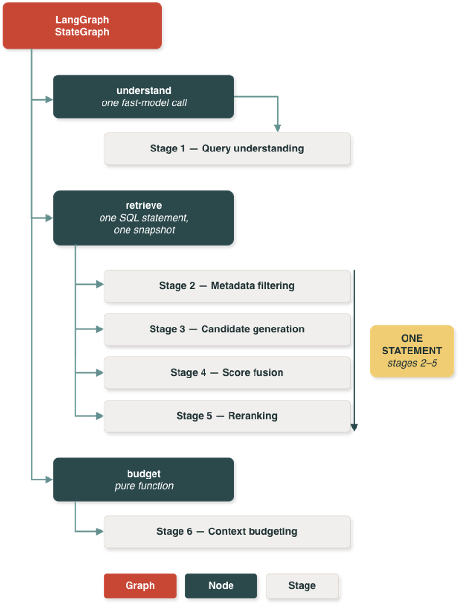
When the pipeline needs observable stages (and in production it does) LangGraph is the better frame. One node per stage, explicit state between nodes, and a graph you can checkpoint and instrument:
from typing import TypedDict
from langgraph.graph import StateGraph, START, END

class RetrievalState(TypedDict):
    query: str
    plan: dict          # stage 1 output: entities, expanded terms, intent, budget
    candidates: list    # stages 2-5 output: reranked, provenance-tagged rows
    working_set: list   # stage 6 output: what Infer & Act consumes

g = StateGraph(RetrievalState)
g.add_node('understand', understand_query)      # stage 1: one fast-model call
g.add_node('retrieve',   retrieve_and_rerank)   # stages 2-5: one SQL statement
g.add_node('budget',     budget_context)        # stage 6: pure function

g.add_edge(START, 'understand')
g.add_edge('understand', 'retrieve')
g.add_edge('retrieve', 'budget')
g.add_edge('budget', END)

retrieval = g.compile()
Notice the graph has three nodes for a six-stage pipeline. Stages 2 through 5 are one node because they are one SQL statement; the database already turned stages 2 through 5 into a single plan. Re-separating them in the orchestration layer would add round trips to recreate a boundary the engine deliberately erased. Oracle AI Database does the retrieval and reranking. LangGraph orchestrates the state around it.
Evaluating retrieval quality
Every number in this article came from somewhere specific, because unmeasured retrieval is unmanaged retrieval. Teams that eyeball a few answers after each change are tuning by anecdote, and anecdotes have terrible recall.
The metrics worth knowing, and why they’re important:
- Recall@k measures how many truly relevant items made the top k. It is the candidate-generation metric. If recall@50 is poor, measure it first and at the fused-candidate boundary because downstream stages cannot recover missing candidates.
- Precision@k measures how many of the top k were relevant. It matters most at the working-set boundary, where every irrelevant item consumes context budget.
- MRR measures how high the first relevant item lands. Use it when one good hit is enough, such as an exact-fact lookup against entity memory.
- NDCG@10 rewards putting the most relevant items highest, using graded rather than binary relevance, over roughly the number of results that fit a context budget. For agent memory retrieval, it captures the ordering that the budget stage consumes. If you track one metric, start with this one.
Warm the reranker before you time it, the same as you would any model server. In recent notebook runs, the first scoring call took roughly 0.9–1.1 seconds. Report that one-time model load separately from warm-path query latency. Assert the range while you are at it. NDCG is normalized to [0, 1], so a value above 1 exposes an evaluation bug, most often an ideal DCG computed from the label list instead of from every gradeable chunk in the corpus. A metric with defined bounds provides a free correctness check on the measurement, and that check is worth more than the metric on the day it fires.
The golden set is the part that sounds hard and isn’t, because the schema already did the work. conversation_memory is the flight recorder: every question, retrieval, answer, and downstream signal (a follow-up, a thumbs-down, a correction) sits in the trace, scoped and timestamped. Log the candidate IDs as a retrieval_result event alongside the tool calls. Harvesting question/relevant-chunk pairs is a query against tables you already operate, followed by a labeling pass where a human (or a strong model, with spot checks) marks which retrieved chunks actually supported a good answer. Two hundred labeled questions can be a useful starting target, but the number you need depends on query variance and the regression size you need to detect. The companion notebook runs on a 36-question demonstration set, which is enough to see a large effect and not enough to split hairs. Production traffic is the test set you already have. You just have to harvest it.
Cadence matters as much as metrics. Once per release is the minimum. On every PR that touches the pipeline is better, and it’s cheap once the golden set exists, because the whole evaluation is a few hundred SQL statements and a scoring script. On every embedding model change it’s mandatory, and this is non-negotiable in a way the others aren’t: new embeddings re-shape the entire vector space, the two-layer article made the derived-layer rebuild an afternoon’s work, and an afternoon is exactly enough time to ship a model that’s better on the benchmark and worse on your corpus without noticing.
LLM-as-judge deserves an accurate framing: it’s a directional signal, useful for catching large regressions between releases and for triaging where to spend labeling effort, and it is not a benchmark. Judges drift with their prompts and inherit the biases of whatever model is judging. Use one to point the flashlight. Use the labeled golden set to make claims.
Beyond hybrid: where agentic retrieval comes in
Everything to this point is one-shot: a question goes in, the pipeline runs once, a working set comes out. The next evolution is agentic retrieval, where the model itself issues queries, reads intermediate results, decides what to fetch next, and stops when it has enough. This is the direction serious production systems are converging, and it reframes classical single-pass RAG as the legacy pattern: not wrong, just the special case where one round trip happens to be enough.
Look back at Jane’s question and you can see why. “What did Letta say about memory eviction, and how does that compare to AgentCore” is two retrievals wearing one question mark. The one-shot pipeline handles it, with the budget stage working to keep both sources represented. An agentic retriever handles it more naturally: query for the Letta paper’s eviction discussion, read the result, notice the paper frames eviction as recursive summarization, then query the AgentCore docs for that specific mechanism, with vocabulary learned from the first result. The second query is better than anything Stage 1 could have written up front, because it was informed by an actual intermediate read.
The part that matters architecturally: agentic retrieval doesn’t replace the hybrid pipeline, it composes it. Every query the model issues (through the retriever tool the LangChain section just built) runs through the same six stages, with the same scope filters, RLS boundary, and reranker. The agent decides what to ask. The pipeline decides what to return, and enforces what may be returned. Getting that separation wrong, letting the model’s queries bypass the pipeline and hit indexes directly, reopens every tenant-isolation hole the schema articles closed.
Cost draws the boundary for when to use it. Each retrieval round is a model call plus a pipeline run, so an N-hop agentic retrieval multiplies both latency and spend by N, and N isn’t known in advance. Compositional, multi-hop, exploratory questions warrant it. “What’s our refund threshold” does not, and an agent that spends four round trips on it is burning money to feel thorough. The practical pattern is an escalation policy: the intent classification from Stage 1 routes simple lookups through one pipeline pass and releases the multi-hop loop only when the question’s structure demands it, under an explicit budget of rounds and tokens.
One question remains open at the end of this pipeline, and it’s the next article. The working set this article produces still has to become a context window, and that assembly (what order, what framing, what gets the model’s strongest attention) is a deterministic construction problem rather than another retrieval problem. There’s a tempting non-answer that would skip it: context windows are a million tokens now, why not retrieve loosely and let the model sort it out? The lost-in-the-middle problem is the counterargument, and the next piece makes it fully: evaluations show that task performance can drop when relevant material sits in the middle of a long context. A larger window changes what fits, while position can still affect performance.
Where this leaves you
The schema articles established tenant-isolated memory with typed records. The two-layer piece separated canonical memory from derived context. This article shows how the agent retrieves from it: filter first, generate vector and lexical candidates, fuse and rerank them, then budget the working set.
If you take one action from this piece, run the ablation yourself. Pull real questions from your traces and hold the model and prompt fixed. Compare the current pipeline against a vector-only baseline, then test hybrid fusion and reranking separately. Measure ranking quality and answer outcomes beside p50 and p95 latency. Keep only the stages that earn their cost on your corpus.
Frequently asked questions
How do I implement hybrid search for AI agent memory?
Apply database-enforced metadata scope first, then generate vector and lexical candidate pools from the allowed rows. Fuse their ranks and optionally rerank the survivors before cutting the result to a context budget. Keep provenance on every returned chunk.
When should hybrid search be used instead of vector search alone?
Test it when queries contain identifiers, error codes, product names, or vocabulary that embeddings tend to blur. Do not assume it wins: on a small corpus with short chunks and a noisy lexical signal, vector search alone may rank better.
How do vector search, lexical search, and metadata filtering work together?
Metadata determines which rows may compete. Vector search finds semantic matches and paraphrases. Lexical search finds exact terms. Rank fusion combines the candidate lists, and reranking can improve their final order.
How do you evaluate whether hybrid retrieval improves AI agent memory?
Build a labeled set from real agent questions and hold the model and prompt fixed. Compare ablations with NDCG and recall, while tracking MRR, answer quality, and p50/p95 latency. Report corpus size and chunking details alongside candidate counts and uncertainty.
What must stay consistent across retrieval stages?
Apply the same authorized scope to vector candidates, lexical candidates, reranking inputs, and cached results. Keep rank scores distinct from permission decisions. Compare the full pipeline with each simpler baseline on exact identifiers, paraphrases, conflicting memories, and no-answer cases.
Continue the implementation: Hybrid Search for Oracle AI Agent Memory: Combining Semantic Recall with Exact Match. Use the validation described above as the acceptance check for your next step.