We use Arm-based processors daily through mobile phones, internet of things sensors, and other devices. Now, this technology has evolved to support data centers and cloud computing. Arm-based processors, including Ampere Altra, scale linearly, provide predictable performance, and provide the highest density of cores, all at a lower price point. Arm is now also being used for high-performance computing applications, such as weather forecasts, drug discovery, and grid management. With Arm-based cloud Compute, customers can run existing workloads at lower costs and build new applications with superior performance.
In this blog, we showcase the performance of SPECFEM3D on Oracle Cloud Infrastructure (OCI) and as compare it to Amazon Web Services (AWS). To know more about why you should use Arm on OCI, see What is Arm?
SPECFEM3D Cartesian simulates fluid, solid, coupled (fluid and solid), or seismic wave propagation in any type of conforming mesh. It models seismic waves propagating based on spectral-element method (SEM) following earthquakes. It can also be used for nondestructive testing or for ocean acoustics.
Setup
OCI offers BM.Standard.A1.160 machines that are Ampere A1 Compute Arm-based standard compute. Each OCPU corresponds to a single hardware execution thread with Ampere Altra Q80-30 processor and max frequency of 3.0 GHz.
| Shape |
OCPU |
Memory (GB) |
Local disk |
Max network bandwidth |
Max VNICs total: Linux |
| BM.Standard.A1.160 |
160 |
1024 |
Block storage only |
2 50-Gbps |
256 |
We created an instance pool of BM.A1.160 machines on OCI using this stack and one of the recommended images.

Figure 1: Compute node options
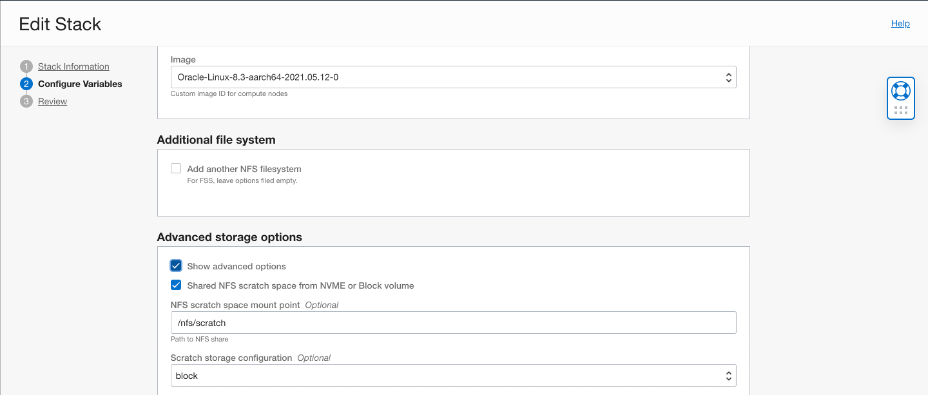
Figure 2: Image and additional file system
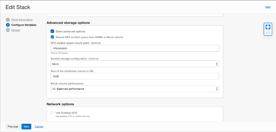
Figure 3: Advanced storage options
For more details on getting started with Arm instances on Oracle Cloud, see the documentation.
Compile SPECFEM3D on OCI Ampere A1
We used the most recent version of SPECFEM3D Cartesian (2.0) from the Git repository and OpenMPI 4.1.0 with Arm Performance Libraries for Linux 21.0, and gcc compiler version 11.1.0.
# git clone --recursive https://github.com/geodynamics/specfem3d.git
# cd specfem3d
# ./configure --prefix=<directory to install>
# make
Run SPECFEM3D on OCI Ampere A1
We’re using a standard model available in the EXAMPLES/meshfem3D_examples/simple_model/ folder.
For both single node and multinode runs, we change the size of the benchmark. Modify the NPROC variable in DATA/Par_file and NSTEP to 5000 and DT to 0.02d0. For each run, modify the value of NPROC, which specifies the number of processors, to 16.
Now update the DATA/meshfem3D_files/Mesh_Par_file to specify the number of grid points in each direction, as shown in the following table. The number of grid points in each direction must be divisible by the number of cores.
| # number of elements at the surface along edges of the mesh at the surface # number of regions 1 256 1 192 5 5 2 1 256 1 192 6 15 3 14 100 7 57 7 10 4 |
OCI results
The following image shows the result of running SPECFEM3D on OCI’s BM.Standard.A1.160 compared to AWS m6g.16xlarge instances from the AWS blog.
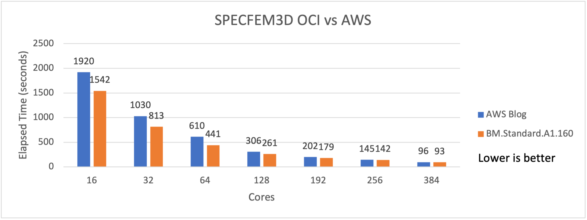
Figure 4: SPECFEM3D OCI versus AWS
We see performance gains of approximately 14% on an average over AWS for a range of 16–384 cores.
In addition, OCI’s BM.Standard.A1.160 is cheaper per SPECFEM3D job than AWS (m6g.16xlarge on-demand pricing in Ohio) on an average of approximately 31% across 64– 384 cores. So, not only are you getting better performance, but you’re cutting costs.
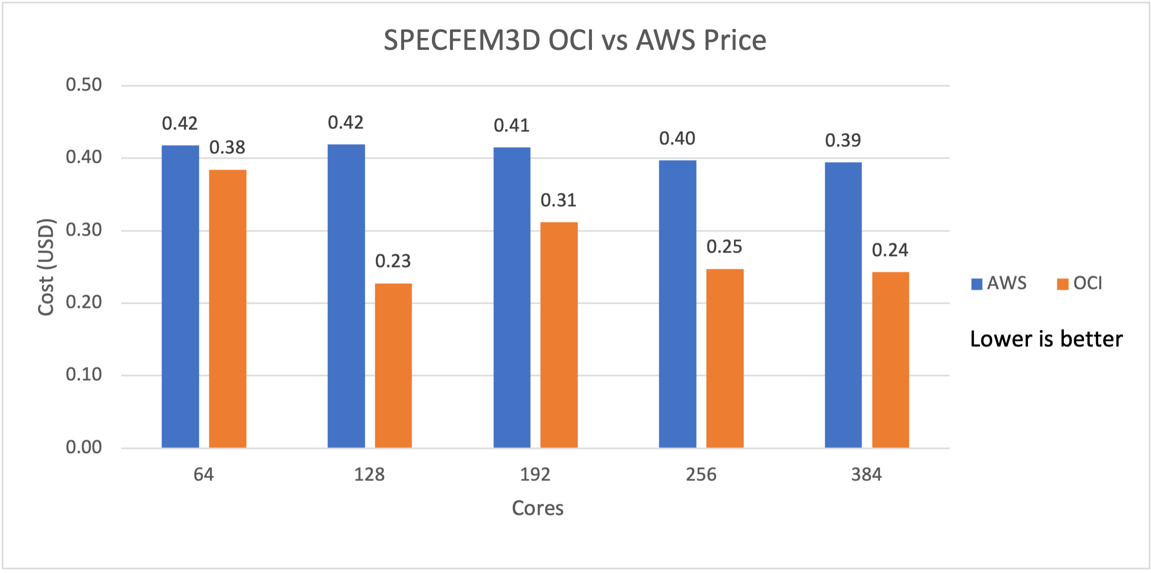
Figure 5: SPECFEM3D OCI versus AWS price

Figure 6: OCI versus AWS on performance versus cost
Virtual machine price comparison
Oracle Cloud also offers virtual machines (VMs) for the Arm processor from Ampere.
| Shape |
Memory per OCPU |
Minimum memory |
Maximum memory |
| VM.Standard.A1.Flex |
64 GB per OCPU |
1 GB or a value matching the number of OCPUs, whichever is greater |
512 GB |
Flexible memory is also available on flexible shapes. The amount of memory allowed is based on the number of OCPUs selected. The ratio of memory to OCPUs depends on the shape. These resources are billed at a per-second granularity with a one-minute minimum. Optimize your costs by choosing the shape that matches your workload.
For example, you can configure the VM to maximize compute processing power by choosing a low core-to-memory ratio. Modify the OCPUs and memory as your workload changes, scaling up to increase performance or scaling down to reduce costs.
For the purposes of calculation for the following comparison, we considered memory according to the following chart.
| Cores |
Memory |
| 16 |
96 GB |
| 32 |
192 GB |
| 64 |
512 GB |
We can optimize the cost further by reducing the memory required by the application.
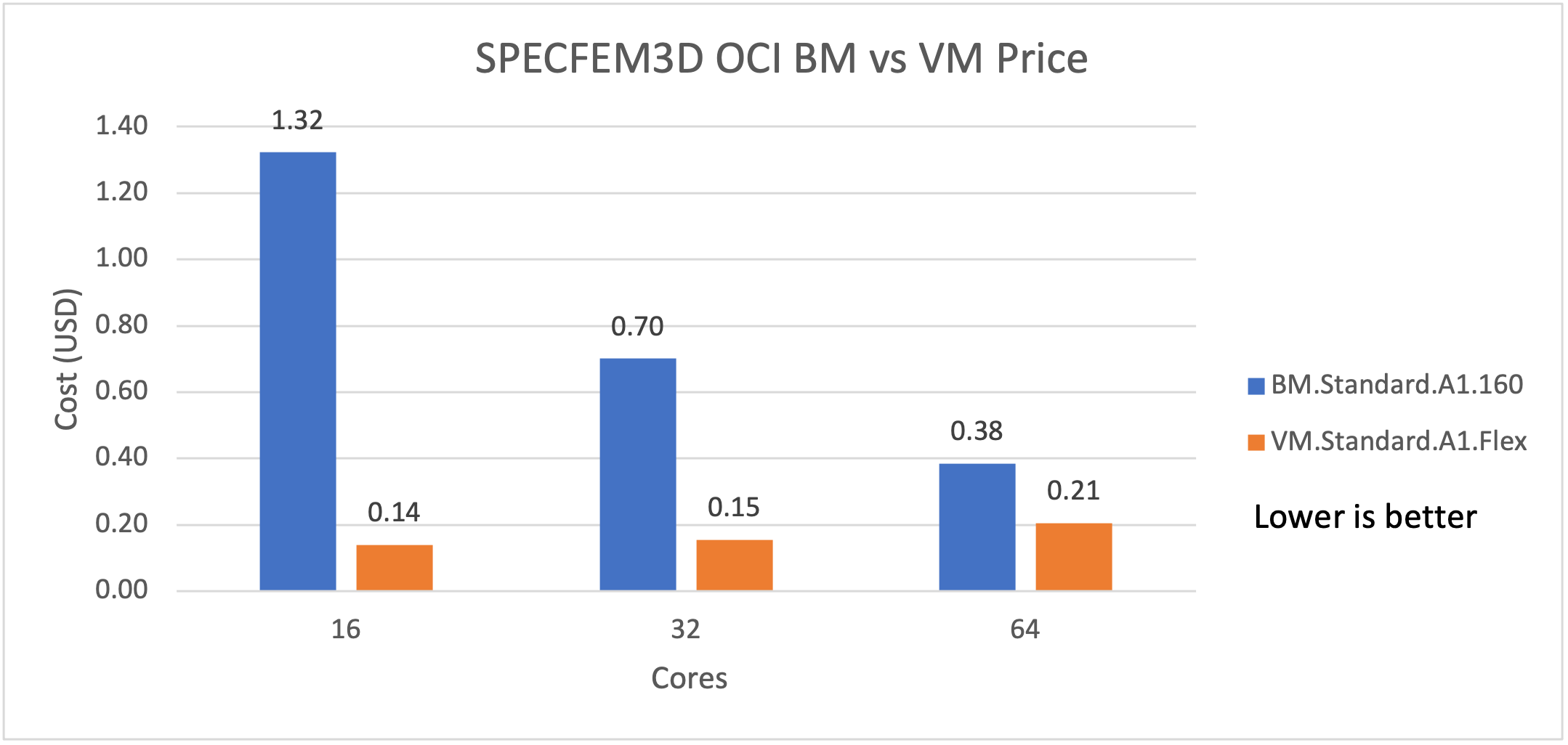
Figure 7: SPECFEM3D OCI bare metal versus VM price
Conclusion
We saw an increase of approximately 14% in performance on BM.Standard.A1.160 compared to AWS, which translates to an average 31% cost savings for your seismic modeling applications. That kind of performance increase leaves no doubt that switching to BM.Standard.A1.160 gives you the best price-performance available in the cloud today. To learn more about how to get started, check out how to start your free 30-day trial today.