Time-series forecasting just got simpler and smarter.
Oracle AI Quick Actions now includes native support for pretrained time-series models, starting with Granite TTM-R1, a compact and high-performing transformer model from IBM. Built for zero-shot forecasting, it’s designed to deliver accurate predictions across a wide range of domains without the need for training. With just a few clicks, you can deploy Granite TTM on Oracle Cloud Infrastructure, stream data to it via API endpoint, and get reliable forecasts for multivariate time-series data without writing any training code. Moreover, TTMs are lightweight and can be executed even on CPU-only machines, enhancing usability and fostering wider adoption in resource-constrained environments.
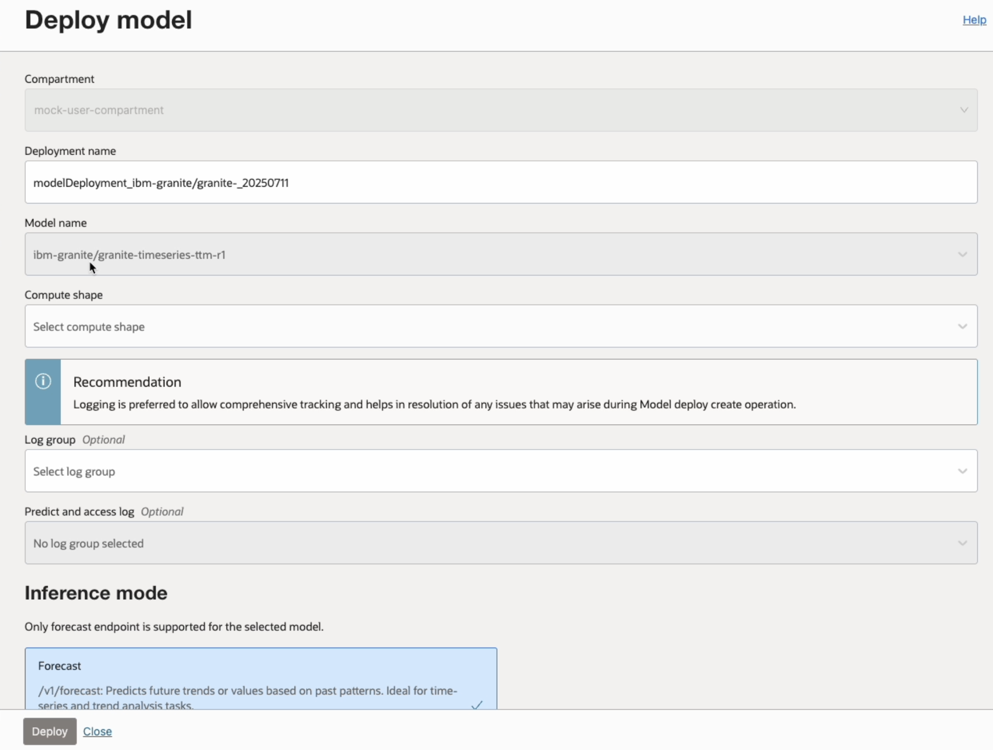
Deploying the Model using AI Quick Action
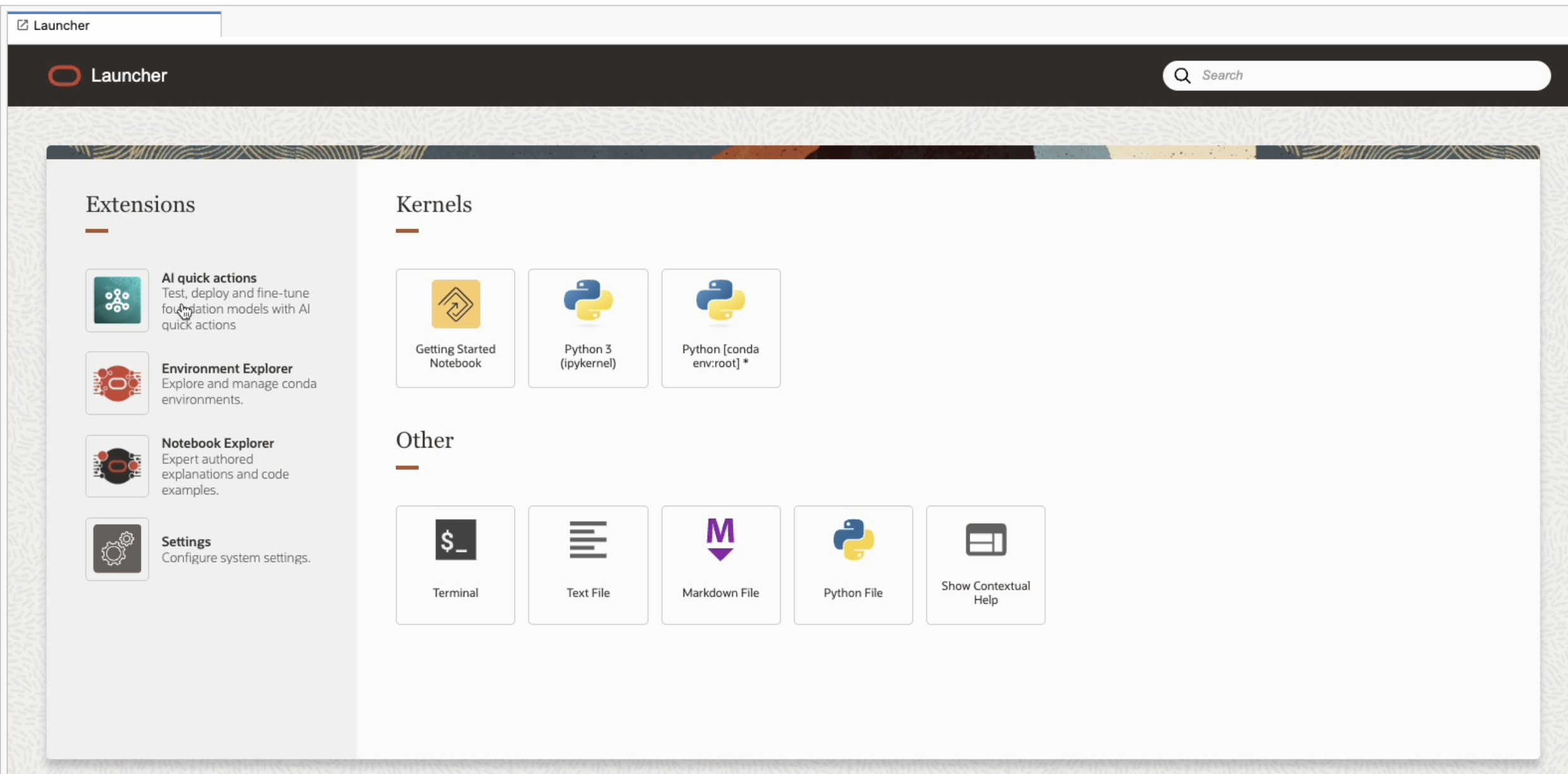
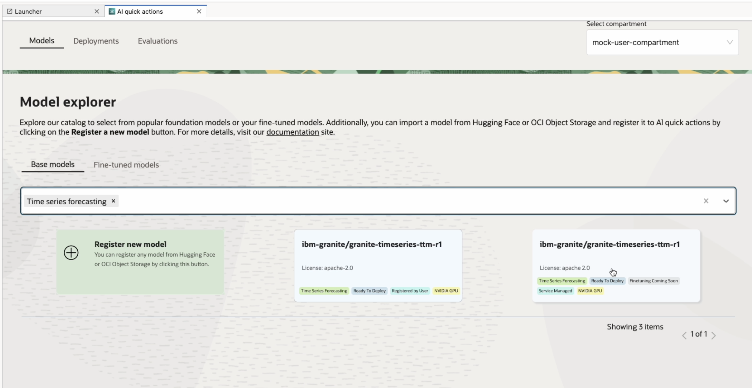
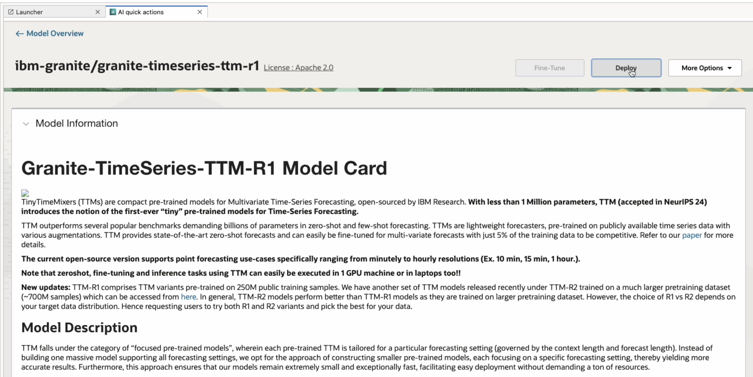
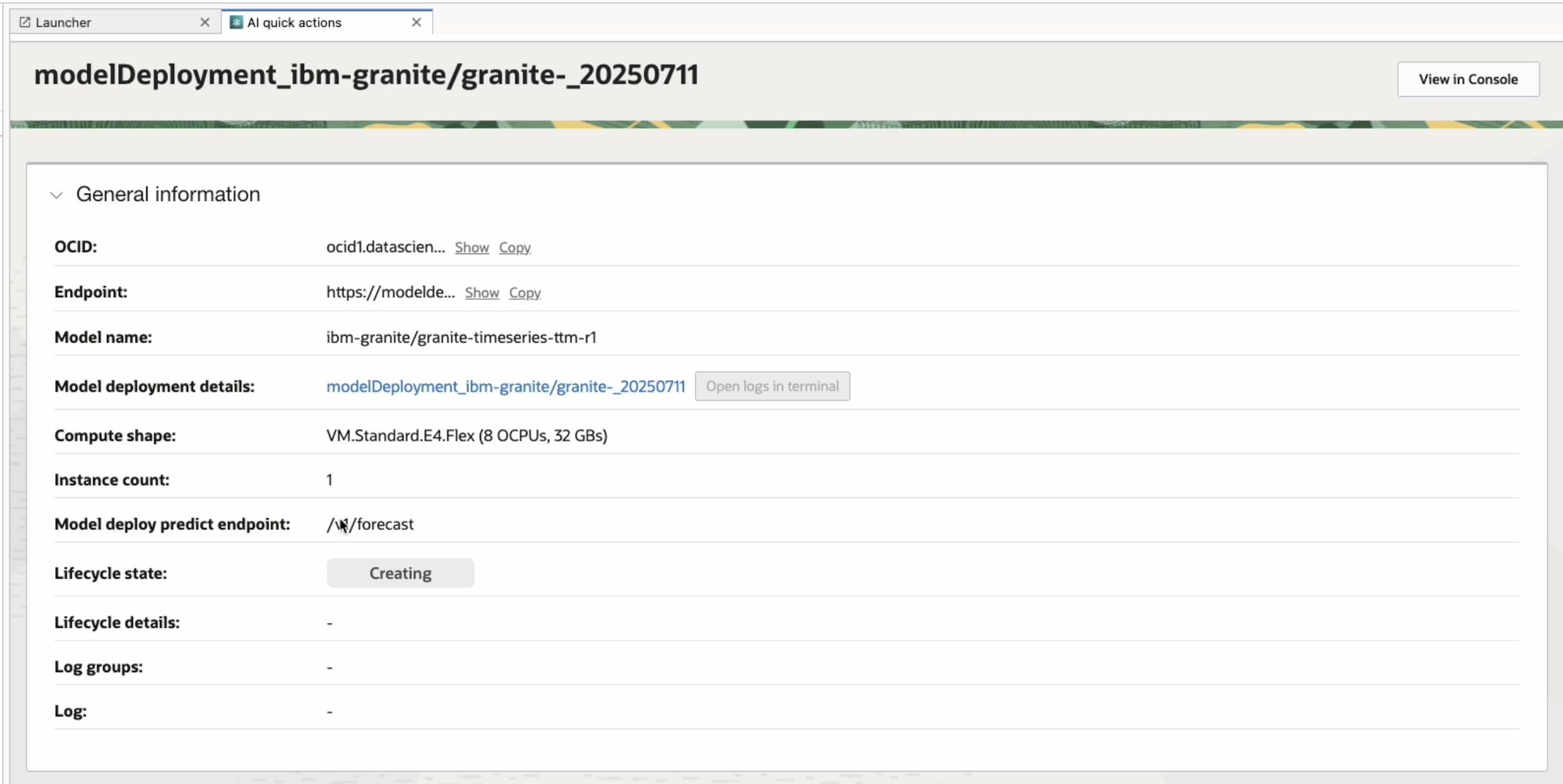
To get started, open AI Quick Actions from the Data Science Notebook and navigate to the Model Explorer. Select the granite-timeseries-ttm-r1 model from the list and click Deploy. Once the deployment is complete, you’ll receive an endpoint URL for making predictions through a REST API. The deployment handles model loading, environment setup, and endpoint exposure automatically.
Once your model is deployed, you’ll receive a REST endpoint for inference. To make a forecast request, simply send a POST request with a properly structured JSON payload. In this example, we use the Seoul Bike Sharing Demand dataset from the UCI Machine Learning Repository.
Preparing the Time-Series Data for Forecasting
import json
import oci
import pandas as pd
import requests

data = pd.read_csv("SeoulBikeData.csv", encoding='unicode_escape')

timestamp_col = "Timestamp"
target_col = "Rented Bike Count"

# data cleaning and preprocessing
data[timestamp_col] = pd.to_datetime(data['Date'] + ' ' + data['Hour'].astype(str).str.zfill(2), format="%d/%m/%Y %H")
data[timestamp_col] = data[timestamp_col].dt.strftime("%Y-%m-%d %H:%M:%S")
data.drop(['Date', 'Hour'], axis=1, inplace=True)
Making a Forecast Request
payload_data = {
    "historical_data": data.to_dict(orient='list'),
    "timestamp_column": timestamp_col,
    "target_columns": [target_col],
    "timestamp_format": "%Y-%m-%d %H:%M:%S",
}
payload_json = json.dumps(payload_data)
# <Provide your endpoint url here >
endpoint = "https://<deployment-host>/ocid1.<deployment-id>/predict"
signer = oci.auth.signers.get_resource_principals_signer()
response = requests.post(endpoint, json=payload_data, auth=signer)
print(response.json())
You’ll get back a JSON response with forecasted values for each target column:
{
  'forecast': [
    {
      'Rented Bike Count_prediction': [
        512.1723122953,
        435.1244180198,
        ..............
        575.5584574211
      ]
    }
  ]
}
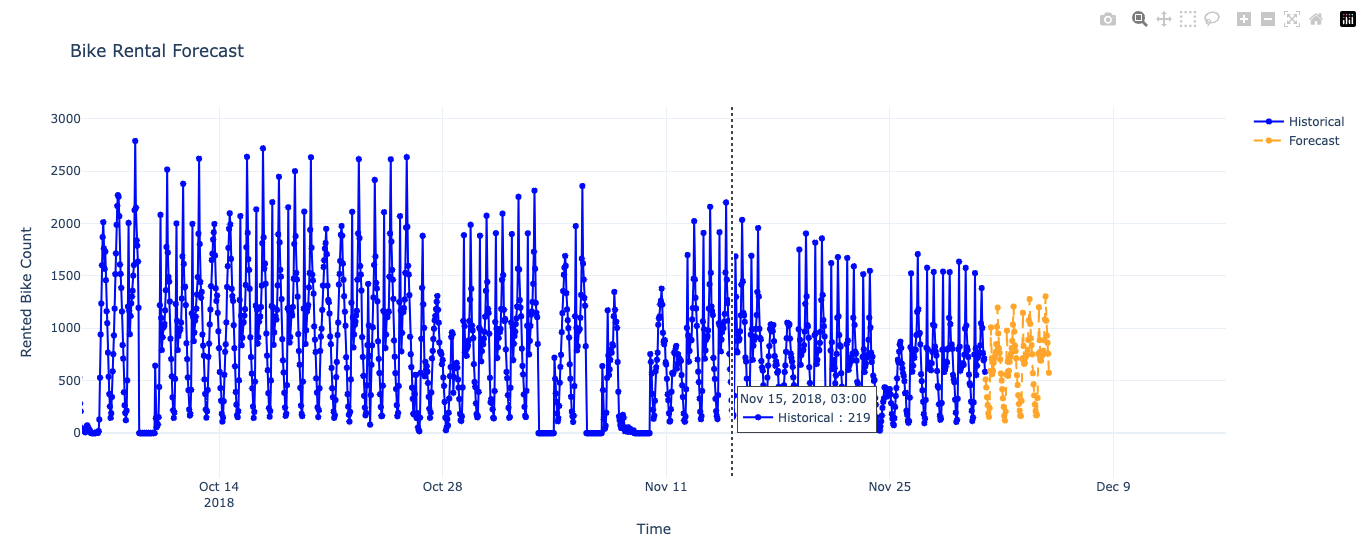
Visualizing the Forecast
from datetime import timedelta
import plotly.graph_objects as go
forecast_dict = dict(response.json())
forecast_values = forecast_dict['forecast'][0][f'{target_col}_prediction']
data['Timestamp'] = pd.to_datetime(data['Timestamp'])
last_timestamp = data[timestamp_col].iloc[-1]
future_timestamps = [last_timestamp + timedelta(hours=i + 1) for i in range(len(forecast_values))]

forecast_df = pd.DataFrame({
    timestamp_col: future_timestamps,
    target_col: forecast_values
})

fig = go.Figure()

fig.add_trace(go.Scatter(
    x=data[timestamp_col],
    y=data[target_col],
    mode='lines+markers',
    name='Historical',
    line=dict(color='blue')
))


fig.add_trace(go.Scatter(
    x=forecast_df[timestamp_col],
    y=forecast_df[target_col],
    mode='lines+markers',
    name='Forecast',
    line=dict(dash='dash', color='orange')
))


fig.update_layout(
    title='Bike Rental Forecast',
    xaxis_title='Time',
    yaxis_title='Rented Bike Count',
    hovermode='x unified',
    template='plotly_white'
)

fig.show()