In this exercise, a historical record of property transactions is loaded into Oracle Autonomous Database (ADB), with Oracle Machine Learning (OML) Notebooks used to prepare that data for ML. We then use the OML AutoML User Interface (UI) to quickly train and optimize a regression model on that data, with that model designed to estimate the market value of any property record. A few APEX dashboards then call that ML model to generate reports and plots of the model’s predictions. The purpose of this walk-through is to illustrate how ADB, OML and APEX can be utilized in concert to make a machine learning task useful and accessible to a broader community of business users via APEX’s point-and-click interface.
OML Notebooks
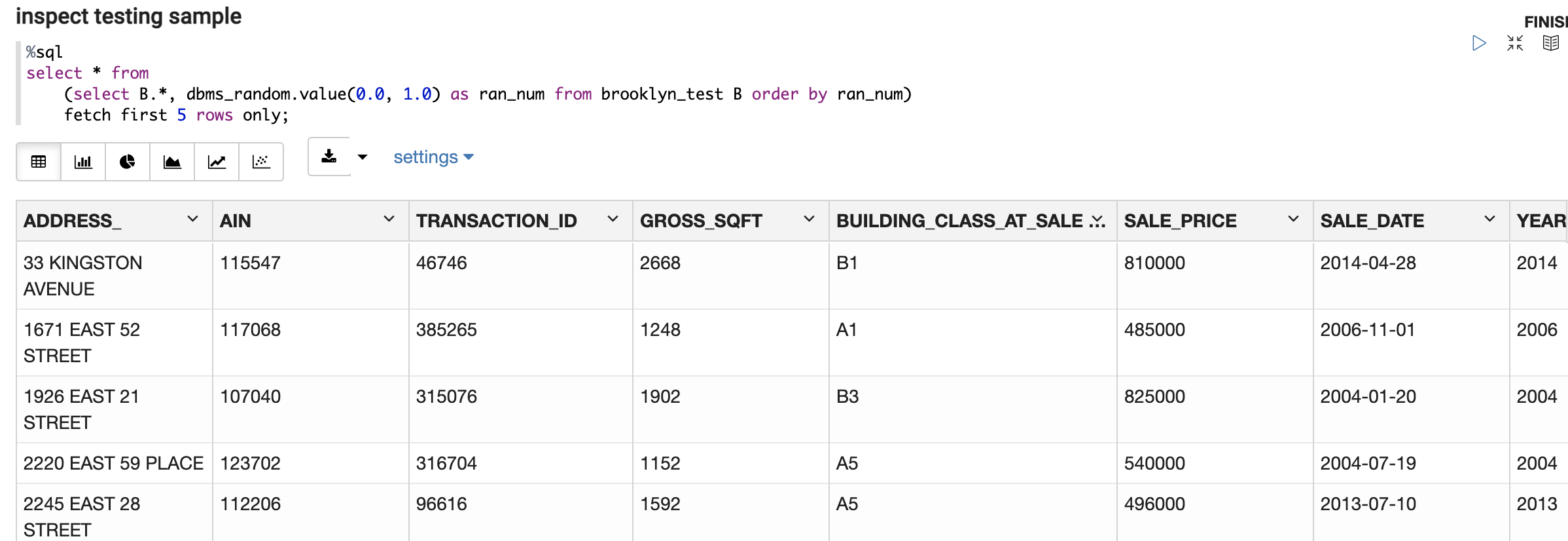
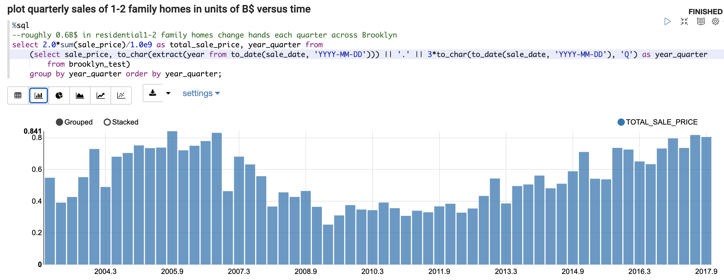
The following will use various OML components provided by Oracle Autonomous Database (ADB) to develop and deploy a machine learning (ML) model. This model will be trained to estimate the market value of residential homes across Brooklyn NY, and that model’s input data is 14 years of Brooklyn property transactions that was originally published by Kaggle that is also mirrored in this Oracle repository. First step is to upload that data into an ADB table, which also makes those records readily available for inspection using Oracle Machine Learning (OML) Notebooks, Figure 1. OML comes with ADB and is a convenient place to develop and debug SQL and PL-SQL code since query results are displayed or visualized inline. OML Notebooks are also fairly language agnostic as it understands R and Python too. OML Notebooks allows us to swiftly develop and spot-check the code that filters and prepares the Brooklyn data that will later be used to train the ML model to predict each property’s market value aka SALE_PRICE. Another great advantage of OML is that, with a click of a button, one can transform a query result into an inline plot, Figure 2. The remainder of the OML notebook shown in Figures 1-2 performs additional filtering and massaging of the input data, and then splits that data into training and testing samples that are stored as ADB tables.
AutoML
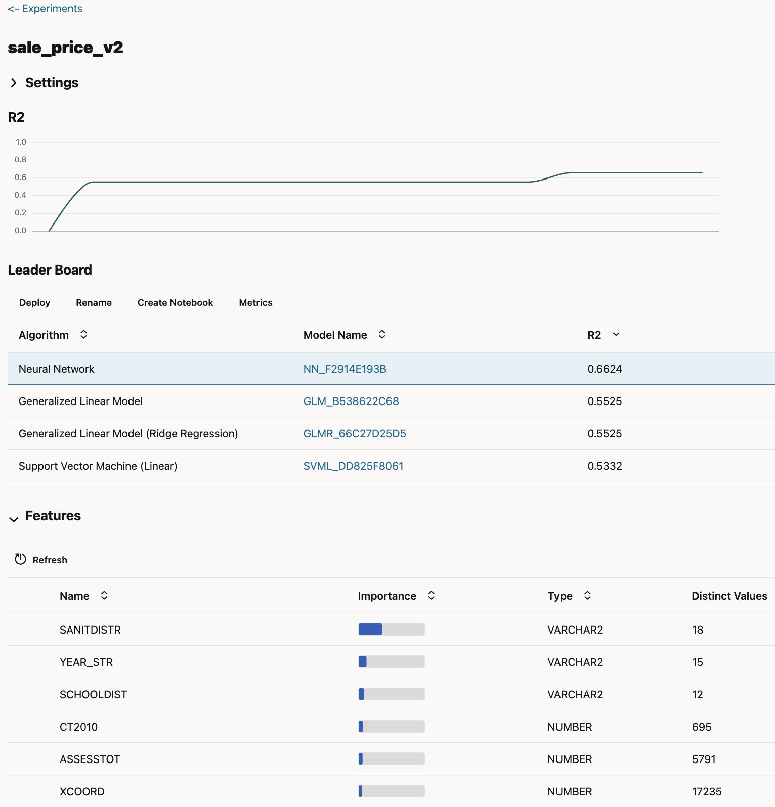
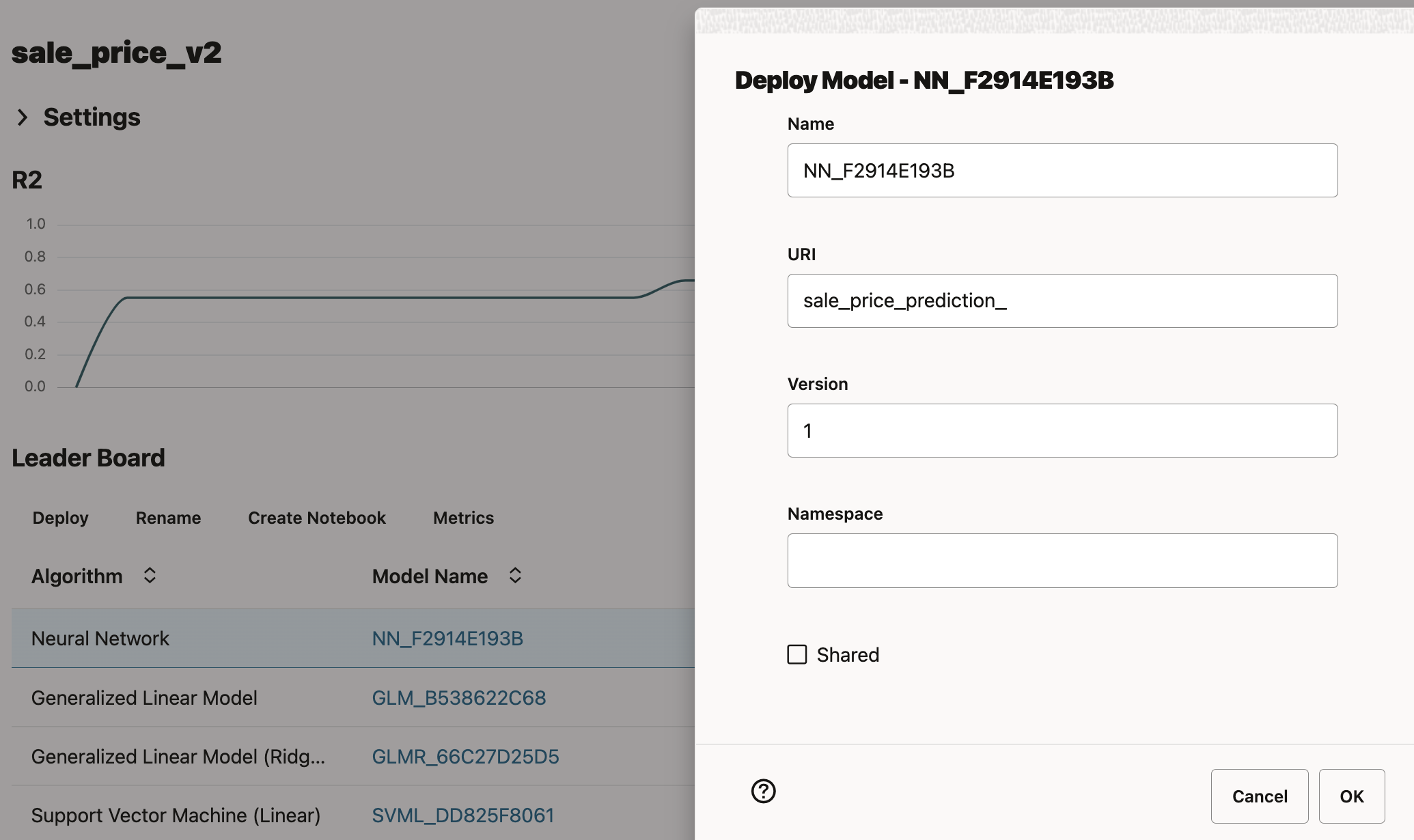
Next, navigate over to the OML AutoML UI where, with a few clicks, we create an experiment that will train a suite of regression algorithms to predict the SALE_PRICE of each of the transacting residences. Pressing the Start button instructs AutoML to evaluate a variety of algorithms used to train ML models: generalized linear regression, ridge regression, linear and nonlinear support vector machines, and a neural network. Note also that if the ADB’s service level is Medium or High, then these models will be trained in parallel on ADB while AutoML automatically tunes their hyperparameters and selects the optimal set of features. After a few minutes we then have a nicely optimized ML model, with Figure 3 showing that the neural network algorithm is the most accurate with an R2=0.66 score. Which is an ok but not a great R2 score, but that is a consequence of this dataset’s slim set of features, which includes some geographic data and a few basic facts about each property (e.g., acreage, home size, and number of floors). Absent are the more granular drivers of home market value such as number of bedrooms, bathrooms, time since last remodel, and any property quality information. If those additional facts were present here, then AutoML would have produced a more accurate model. Nonetheless the current model is good enough to demonstrate ADB’s MLOps capability, which is the main goal of this exercise.
Figure 3 also shows that AutoML provides a ranked list of optimized models and their model names. This is useful because these models are first-class database objects that any database user, code, or OCI service (such as Oracle Analytics Cloud OAC) can access via SQL to generate a model prediction. This means that any ML model trained on ADB is also instantly deployed, since any other user/code/service having access to that database can also interact with that model and benefit from its predictions.
OML4Py
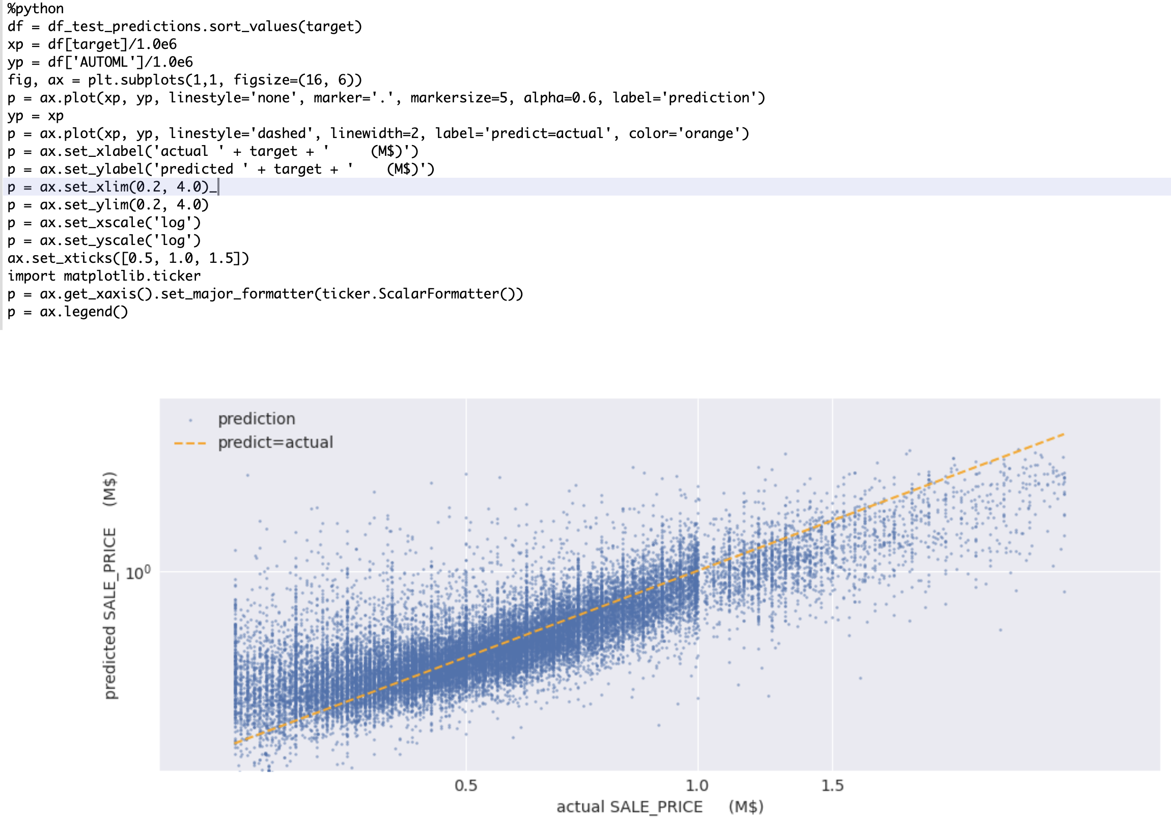
Next, highlight the highest-ranking neural network model seen in Figure 3 and click Create Notebook, which generates a new OML notebook with OML4Py code that will rebuild the neural network model using the same training data and tuned hyperparameters (Figure 4). This allows the user to tailor that model further if desired, and to generate additional model validation plots like Figure 5. A noteworthy advantage of the OML4Py library is that it allows a Python user to establish pointers to database tables that can then be manipulated further (e.g., filters, joins, aggregations, etc.) via straightforward Python code. So if you find yourself struggling to compose or debug deeply nested SQL code that is challenging to understand or maintain, consider recasting that complex SQL into easy-to-read Python via the OML4PY library.
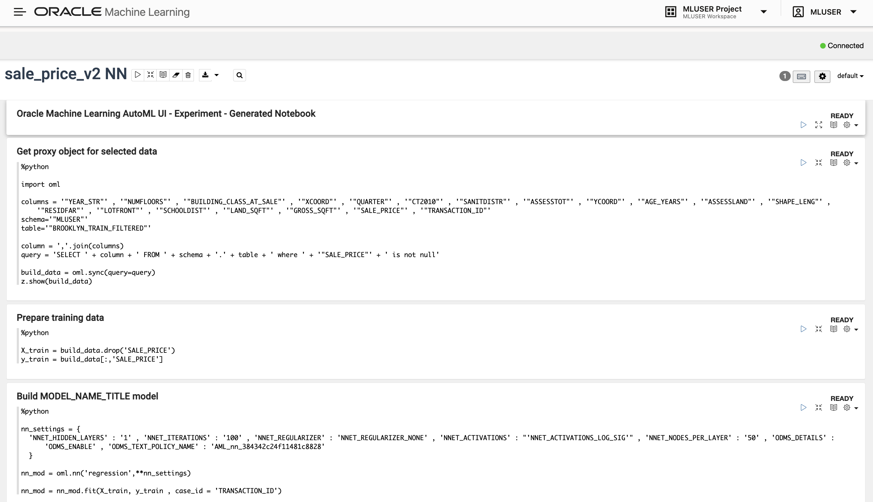
Figure 5 also uses OML’s custom Python ability to plot the neural network model’s predicted SALE_PRICE versus each property’s actual SALE_PRICE. Note that this scatterplot shows that model estimates are ‘too warm’ for very low-end properties, and that model estimates are ‘too cool’ when estimating the market value of the highest-value properties. This behavior is in fact typical of all ML models, and this issue will be addressed later when we use APEX to perform ‘edge-trimming’ of some of these predictions.
Model Deployment
The OML AutoML UI also makes the deployment of an ML model as a REST endpoint especially easy. Again, highlight the highest-ranking neural network model shown in Figure 3, click Deploy, and then provide that deployment’s URI which in this example will be sale_price_prediction (see Figure 6), then click OK to deploy that ML model.
Our next task is to confirm that we can programmatically interact with that deployed model’s API, which is the most challenging portion of this walk-through, but straightforward nonetheless.
Testing the Deployment
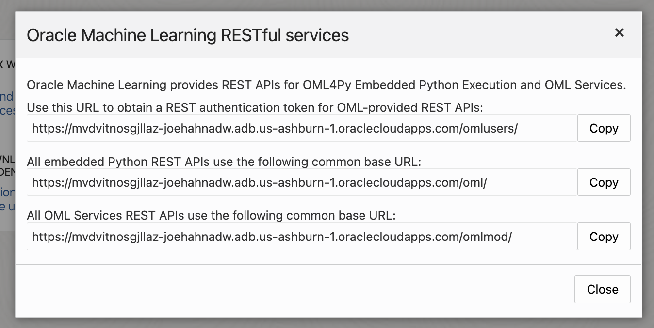
Begin the test by using the OCI console page to start a cloud shell session. Then navigate to ADB > Database Actions > OML RESTful services and copy the first url such as that seen in Figure 7. Navigate back to the cloud shell session and paste that url into a shell variable called token_server_url, with “api/oauth2/v1/token” also appended such that our revised token_server_url has this form:
token_server_url=https://mvdvitnosgjllaz-joehahnadw.adb.us-ashburn-1.oraclecloudapps.com/omlusers/api/oauth2/v1/token
An accessToken is required when interacting with the deployed model’s REST API, and that accessToken is requested via this call to token_server_url:
curl -X POST –header ‘Content-Type: application/json’ –header ‘Accept: application/json’ -d ‘{“grant_type”:”password”, “username”:”‘<username>'”, “password”:”‘<password>'”}’ “${token_server_url}”
where <username> and <password> refer to our ADB user credentials. The above then displays a 985-character-long accessToken that is stashed in another shell variable
accessToken=’eyJhbGciOi… h2H4Ca2w==’
that is shortened here for brevity.
The deployed model’s scoring URL is also inferred from the third URL seen in Figure 7 followed by the model’s deployment_uri (Figure 6):
score_url=”https://mvdvitnosgjllaz-joehahnadw.adb.us-ashburn-1.oraclecloudapps.com/omlmod/v1/deployment/sale_price_prediction/score”
We then feed the accessToken plus a property’s relevant facts into the scoring URL via
curl -X POST –header “Authorization: Bearer ${accessToken}” –header ‘Content-Type: application/json’ “$score_url” -d ‘{“inputRecords”:[{“YEAR_STR”: “2016”, “NUMFLOORS”: 2.0, “BUILDING_CLASS_AT_SALE”: “B1”, “XCOORD”: 1012437, “QUARTER”: “3”, “CT2010”: 974.0, “SANITDISTR”: “18”, “ASSESSTOT”: 38376, “YCOORD”: 175458, “AGE_YEARS”: 17, “ASSESSLAND”: 9088, “SHAPE_LENG”: 263.108470427, “RESIDFAR”: 1.25, “SCHOOLDIST”: “18”, “LAND_SQFT”: 2858, “GROSS_SQFT”: 4818}]}’
which responds with
{
“scoringResults”: [
{
“regression”: 800205.4431348437
}
]
}
which tells us that this particular 17-year-old two-story house had an estimated market value of about $800K during the 3rd quarter of 2016.
This confirms that one can use custom code to interact with the deployed model’s REST API. Which would be handy if one wanted to use code to embed an ML model’s predictions into a data-handling pipeline or application. But the above can be inconvenient when a person wants to interact with the ML model, and for those interactions we pivot to the APEX service that is also provided by ADB.
APEX
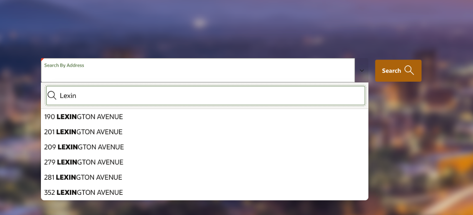
After we have deployed the ML model that estimates the market value of residential properties across Brooklyn NY, APEX is then used to quickly build an application that will use that ML model to generate predictions. APEX is Oracle’s low-code application development tool, and it interoperates with any version of the Oracle Database including ADB. Using APEX’s wizard-driven interface, we first create a search page that will display the details of any Brooklyn property record that exists in the ADB database instance, Figure 8.
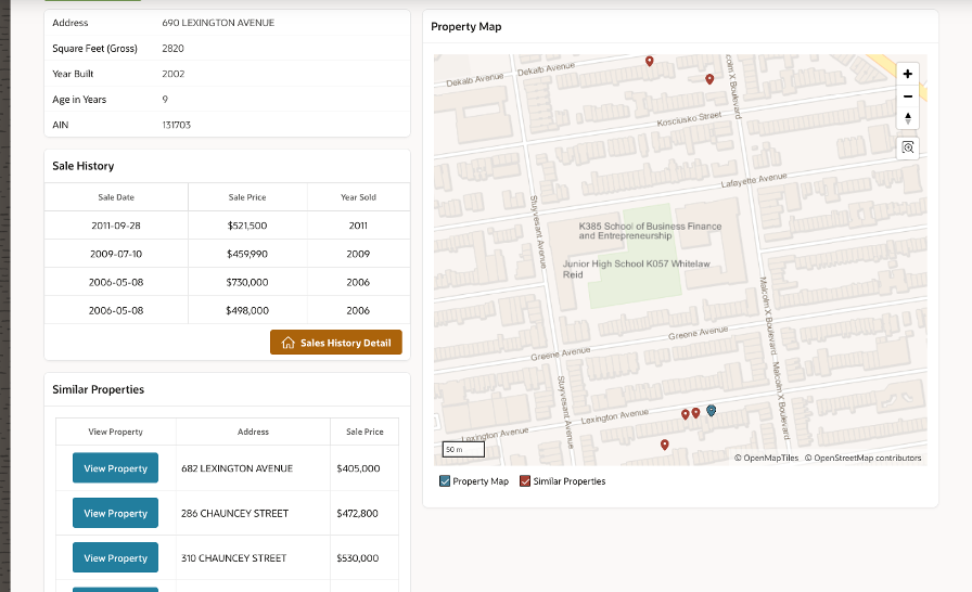
Searching for a Brooklyn address then brings up a short report showing that property’s sale history, as well as an interactive map showing that property’s location, Figure 9. That report also uses the ML model to compute on-the-fly the market values of the desired property’s ‘comps’, which are other properties in the vicinity having similar features.
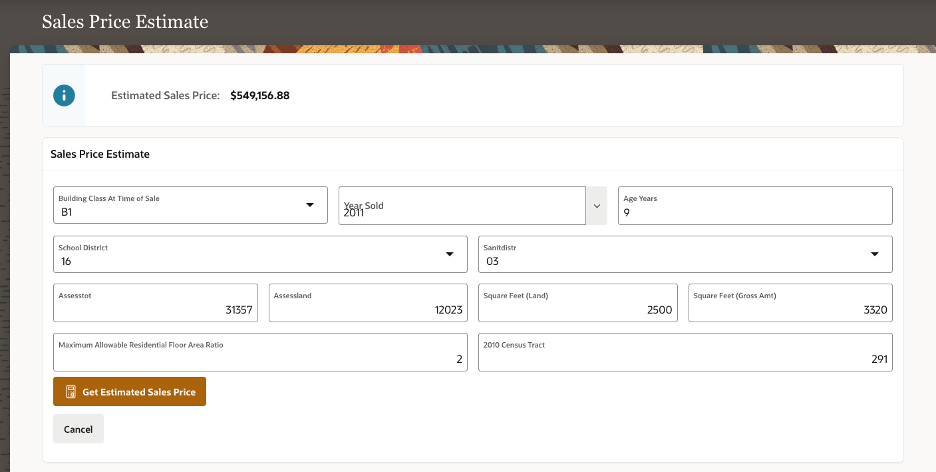
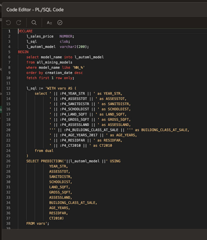
The next APEX dashboard, Figure 10, allows the user to perform “what-if” scenario analysis. That dashboard permits the user to adjust a given property’s attributes to account for potential changes to that residence, such as for example adding 500 square feet to the property’s home. Changes made via the APEX interface then triggers a call to the ML model that provides a revised estimate of the property’s market value. Figure 11 also peeks under the APEX hood to show how the APEX Page Designer interface allows the user to embed the custom SQL and PL-SQL code that the APEX dashboard uses to call the ML model, which in turn enables the interactive what-if analysis seen in Figure 10.
Maps
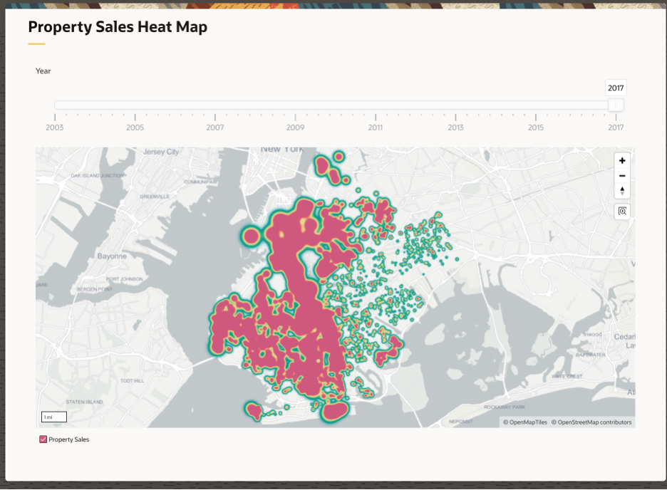
One of APEX’s more powerful capabilities is its mapping ability. Whether using simple latitude/longitude coordinates, Oracle Database’s native SDO_GEOMETRY, or GeoJSON data, the Maps feature of APEX makes it easy to create heat maps, and Figure 12 uses the properties’ latitude/longitude coordinates to heat-map their market value across Brooklyn.
Model Retraining
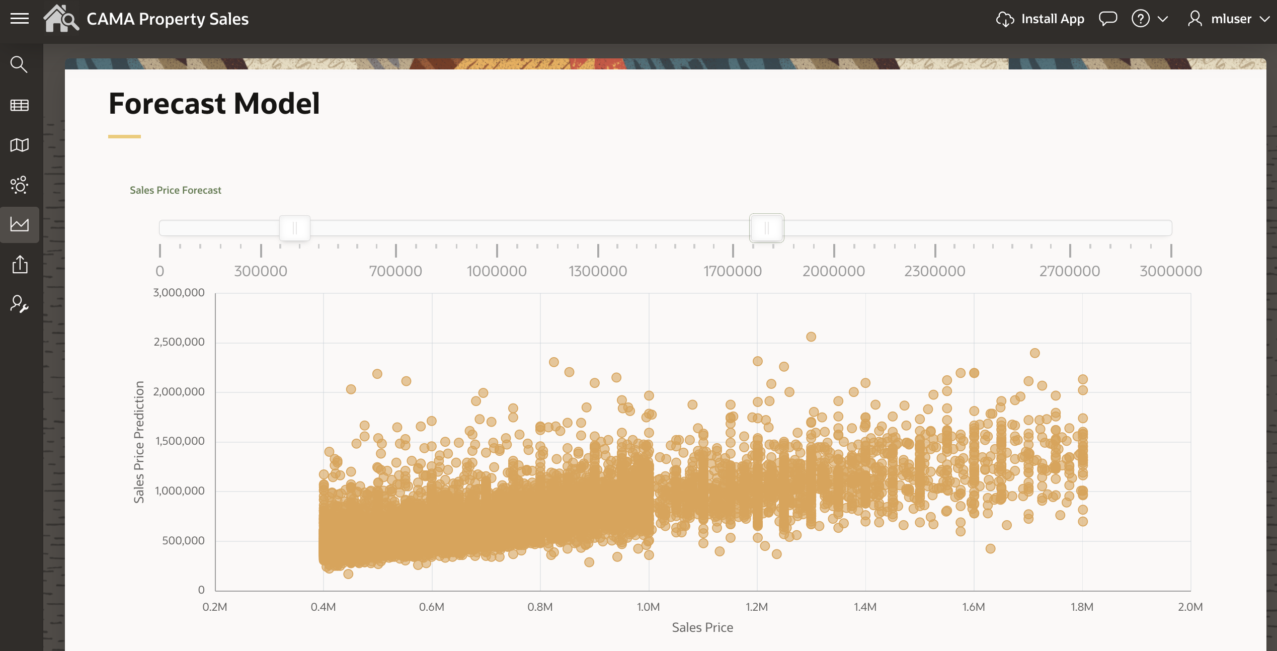
APEX coupled with Oracle Database also allows us to identify and filter out any spurious records that might exist in the ML model’s training sample. Recall that Figure 5 shows that the current ML model performs poorly for very low-end properties having SALE_PRICE < $450K as well as for high-end properties having SALE_PRICE > $1.1M. Point is, it is often desirable to filter outlier records from the training sample and then retrain the model using a more performant training data. This possibility is illustrated in Figure 13, which uses a slider plus an interactive scatterplot to allow the APEX user to drop the undesired low and high-end properties, all of which are enabled by an APEX dynamic action that filters the training sample via custom PL/SQL in the backend.
Main Findings
APEX is a powerful low-code application development tool that is well-suited for exposing Oracle Database data and functionality, including machine learning, to business users via dashboards that are tailored to those users’ needs. As this walk-through shows, impactful results are possible when APEX is utilized in concert with OML, which was used here to prepare database data, and with the OML AutoML UI to train the ML model with push-button ease, with those model predictions then made actionable via APEX’s point-and-click interface.
Possible Next Steps
The motivated reader is also encouraged to rebuild the above in their Oracle Cloud Infrastructure (OCI) tenancy. There one can launch an ADW instance within the Oracle cloud, load the Brooklyn property data into an ADW table, use the OML AutoML UI to train and deploy the ML model, and then use APEX to visualize those model predictions. This exercise’s OML notebooks and APEX application are also archived at this code repository.
For more information about the topics mentioned in this blog post, please consult these resources: