In this post, we will explore how to solve optimization and scheduling problems using techniques from Operations Research, Linear Programming, and Python.
Next, we will use Oracle Machine Learning to develop and run these algebraic models in agribusiness.
Introduction
In this article, we will explore a typical optimization problem that can be addressed using Operations Research techniques. As an example, we will plan the planting of three different crops to optimize profit.
But what exactly is Operations Research?
Operations Research
Operations Research, or OR, is a discipline that utilizes analytical methods for complex decision-making. The goal is to transform real-world problems into mathematical models to identify an optimal solution for a defined objective and set of constraints.
Officially, OR emerged during World War II due to the need to optimize the scarce resources of military forces, such as the size of naval convoys and bomber tactics.
The idea of OR is to minimize, maximize, or find an exact value for an objective function, based on a set of constraints.
Among many techniques within Operations Research, we can mention linear, integer/mixed programming, and simulations, among others.
Linear programming consists of three main elements: decision variables, an objective function, and constraints, which in this example will be modeled using the PuLP library and solved with the CBC Solver that comes integrated with it.
In this example, we will adopt linear programming using the Python language along with the aforementioned PuLP library, all running within Oracle Machine Learning.
About Oracle Machine Learning
Oracle Machine Learning, or OML, is an embedded solution that comes with the Oracle Autonomous AI Database and focuses on creating and deploying machine learning models directly within the database. With this, among many other advantages, we can process analysis and predictions directly in the database without data export or movement.
OML supports development in Python, R, and SQL, as well as no-code tooling and AutoML, which automates several stages of the model creation process, such as algorithm selection or hyperparameter tuning.
The solution allows for the creation of custom Conda environments—which we will do in this article, since we need a library called PuLP that is not standard in OML—and enables the execution of the Jupyter/Zeppelin notebook created during the modeling process as a job, in order to perform inference directly within the database. The entire mathematical modeling process and solver execution for our study will run within Oracle Machine Learning.
There will be no machine learning model training, since the category of problem we are solving involves Linear Programming. Instead, our work will consist of defining decision variables and creating the objective function we want to maximize along with its constraints.
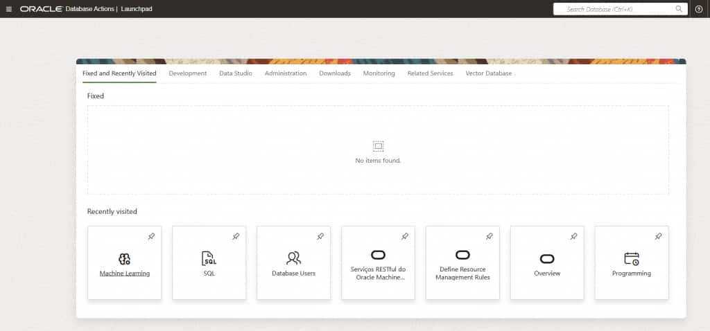
Oracle Machine Learning, or OML, can be accessed via the Launchpad under Database Actions on the Oracle Autonomous AI Database page. OML needs to be activated on the main Oracle Autonomous AI Database page; if everything is set up correctly, it will appear as the Machine Learning option shown below.
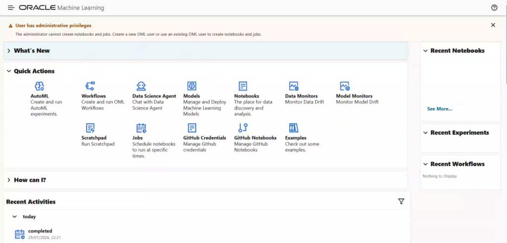
On the OML screen, the ‘Quick Actions’ section displays several options focused on creating machine learning algorithms, workflows, agents, jobs, and model deployments, among many other features. Here, two options interest us: the first is ‘Notebooks,’ where we will create the optimization algorithm, and the second is ‘Jobs’ to execute this algorithm at regular intervals.
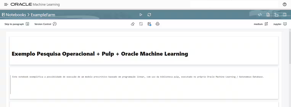
The Oracle Machine Learning Notebook can be either Jupyter or Zeppelin. The important thing here is the ability to use the data available in the Oracle Autonomous AI Database to train machine learning models or develop advanced analytical work without the need for data movement.
After this brief overview of OML, let’s talk a little about the Python library that allows us to solve a linear programming / optimization problem.
Pulp Library
OK, so far we have talked about Oracle Machine Learning, Linear Programming, and Operations Research, but what is the role of this library called PuLP?
Basically, the library is a linear programming modeler that allows us to define optimization problems and solve them by calling solvers like CBC, Gurobi, and CPLEX. Notice that these are two separate components: PuLP, in its role as a modeler, allows us to write the definition of the problem with all its constraints, the objective function definition, and variables.
However, this definition alone is not enough. It is necessary to use a solver to execute this definition and receive the optimized values. Solvers are mathematical optimization tools focused on solving complex problems. A typical definition begins with:
# 1 - Import PuLP modeler functions
from pulp import *

# 2 - Problem to be solved
prob = LpProblem("The Whiskas Problem", LpMinimize)

# 3 - Variables Definition
x1 = prob.add_variable("ChickenPercent", 0, None, LpInteger)
x2 = prob.add_variable("BeefPercent", 0, None, LpContinuous)

# 4 - Objective Function
prob += 0.013 * x1 + 0.008 * x2, "Total Cost of Ingredients per can"

# 5 - Constraints
prob += x1 + x2 == 100, "PercentagesSum"
prob += 0.100 * x1 + 0.200 * x2 >= 8.0, "ProteinRequirement"
prob += 0.080 * x1 + 0.100 * x2 >= 6.0, "FatRequirement"
prob += 0.001 * x1 + 0.005 * x2 <= 2.0, "FibreRequirement"
prob += 0.002 * x1 + 0.005 * x2 <= 0.4, "SaltRequirement"

# 6 - Solver execution
prob.solve()
With this, we obtain an optimal solution for the defined model. Now, let’s talk specifically about the optimization problem that we want to solve in this exercise.
Describing the Case
AgroFuturo Farm has a total area of 10,000 hectares available for the next agricultural cycle. The producer wishes to plant three crops: Soybeans, Corn, and Cotton. The objective is to determine how many hectares of each crop to plant in order to maximize the total net profit, while respecting the following business conditions:
Financial Return (Net Profit per Hectare):
SoyBeans: R$ 3.000 / hectare.
Corn: R$ 2.000 / hectare.
Cotton: R$ 4.500 / hectare.
Crop Rotation and Soil Restrictions:
To preserve soil nutrients, the Corn area must be at least 20% of the total planted area.
Rainfall Forecast Restriction (Water Consumption):
The meteorological report indicates a critical limit for available irrigation/water for the harvest. The water consumption per hectare (in irrigation units) is: Soybeans = 2 un/ha, Corn = 1 un/ha, Cotton = 3 un/ha. The total water availability is 22,000 units.
Machinery Limit Restriction (Harvesting Time):
Cotton requires a significant amount of time from the farm’s exclusive harvesters. Due to the limited fleet, the producer can harvest a maximum of 2,500 hectares of Cotton this season.
Forward Sale Contract Restriction:
The farm has signed an advance contract and must strictly deliver the production equivalent to at least 1,500 hectares of Soybeans.
Mathematical Formulation
Decision Variables:
Represent what the producer needs to decide (in hectares):
x1: Area to be planted with Soybeans
x2: Area to be planted with Corn
x3: Area to be planted with Cotton
2. Objective Function
The goal is to maximize the total profit:
Maximize Z=3000×1+2000×2+4500×3
3. System Constraints
- Available Land Limit: The sum of the planted areas cannot exceed 10,000 hectares.
x1+ x2 +x3 <= 10000 - Crop Rotation (Minimum Corn): Corn (x2) must be at least 20% (0.2) of the total planted area (x1 + x2 + x3).
x2 >= 0.2(x1+ x2 + x3)
- Water Availability (Rainfall/Irrigation):
2×1+1×2+3×3 <= 22000
- Machinery Capacity (Maximum Cotton):
x3 <= 2500
- Futures Contract (Minimum Soybean):
x1 >= 1500
- Non-Negativity: There is no planting of negative areas.
x1,x2,x3 >= 0
Solving Optimization Problems with Oracle Machine Learning
For this category of problem we don’t need to train a new machine learning model, but we define an algorithm using linear programming, a Jupyter Notebook from OML and Python.
Before coding our algorithm we need to mount the Conda environment with our dependencies and mainly the PuLP library. To mount this environment we need to make use of following instruction
%conda create -n mypyenv python=3.10 pulp
After that, we have a Conda environment, but we need to download and activate this environment with:
%conda
download mypyenv
activate mypyenv
The code below implements the main topics of a typical optimization problem: begin declaring the problem, the decision variables and the objective function. Then we insert the constraints and finish solving the problem.
The result provides the optimal planted area for each crop under the model’s assumptions and the corresponding estimated objective value.
import pulp

# 1. Create the maximization problem
pobl = pulp.LpProblem("Otimizacao_Uso_do_Solo_Agro", pulp.LpMaximize)

# 2. Define Decision Variables (hectares)
# lowBound=0 sets the lower bound to zero / non-negativity constraint
x1 = pulp.LpVariable("Soja", lowBound=0, cat="Continuous")
x2 = pulp.LpVariable("Milho", lowBound=0, cat="Continuous")
x3 = pulp.LpVariable("Algodao", lowBound=0, cat="Continuous")

# 3. Define the Objective Function (Maximize Net Profit)
pobl += 3000 * x1 + 2000 * x2 + 4500 * x3, "Lucro_Total"

# 4. Insert System Constraints
pobl += x1 + x2 + x3 <= 10000, "Limite_Terra"
pobl += -0.2 * x1 + 0.8 * x2 - 0.2 * x3 >= 0, "Rotacao_Culturas_Milho"
pobl += 2 * x1 + 1 * x2 + 3 * x3 <= 22000, "Disponibilidade_Agua"
pobl += x3 <= 2500, "Capacidade_Maquinario_Algodao"
pobl += x1 >= 1500, "Contrato_Futuro_Soja"

# 5. Solve the model
pobl.solve()

# 6. Show the Optimized Results
print(f"Solver Status: {pulp.LpStatus[pobl.status]}")
print(f"Ideal Area for Soybean: {x1.varValue:.2f} hectares")
print(f"Ideal Area for Corn: {x2.varValue:.2f} hectares")
print(f"Ideal Area for Cotton: {x3.varValue:.2f} hectares")
print(f"Total Planted Area: {x1.varValue + x2.varValue + x3.varValue:.2f} hectares")
print(f"Maximum Estimated Profit: R$ {pulp.value(pobl.objective):,.2f}")
This very simple script represents an optimization model with a few constraints written directly in code, although they could be parameterized in the database, along with the decision variables and other elements.
Executing it from the notebook allows us to not only run the executable code in Python, R, or SQL, but also describe the experiment in detail, fully outlining the problem, its mathematical formulation, and the modeling stages. Notice that this goes far beyond a simple code comment.
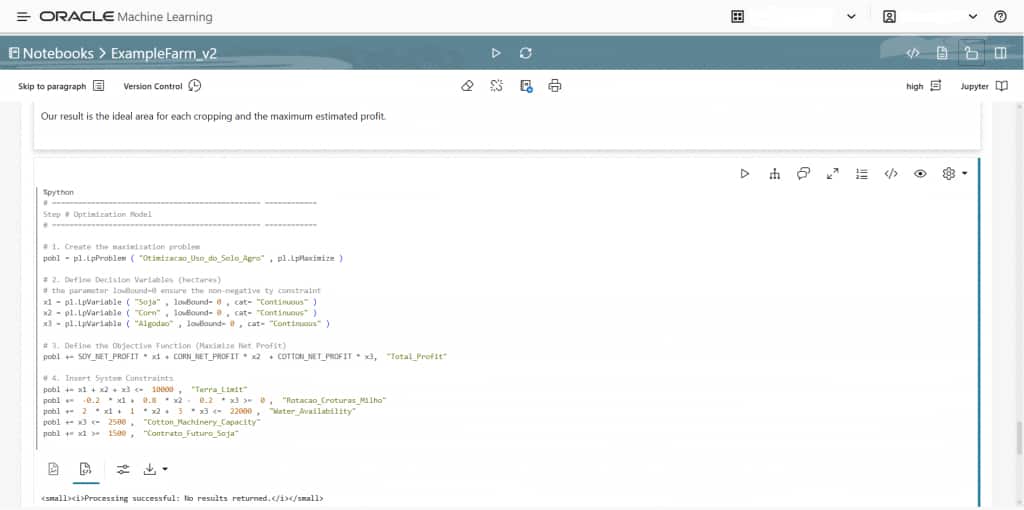
The image above show the necessary steps to define an optimization model. After that, we can solve the objective function and get the optimized values.
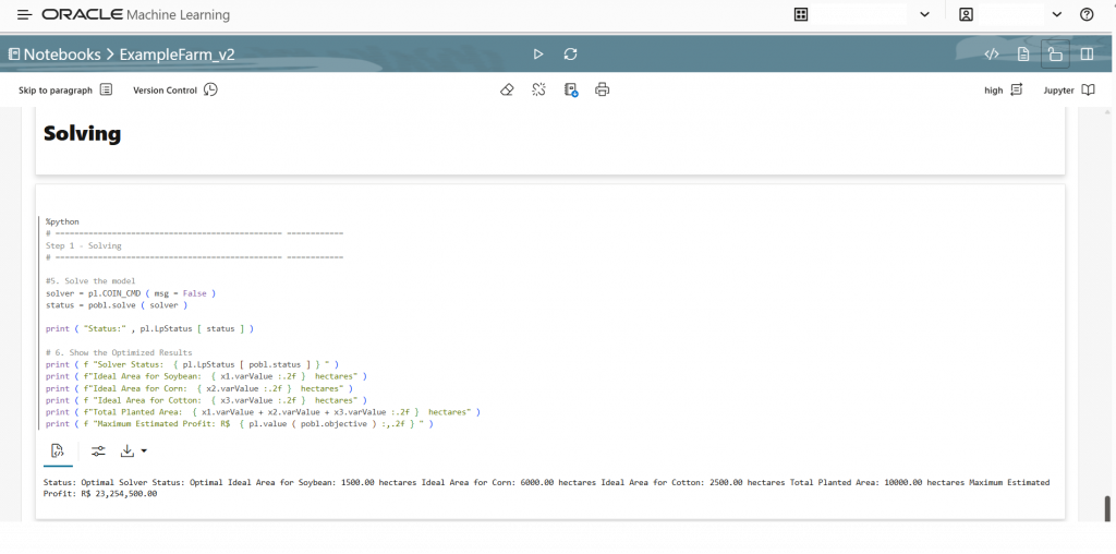
We ask the model to maximize estimated profit based on the defined inputs and constraints, and it returns the optimal allocation under those assumptions. Now we need to schedule the notebook execution.
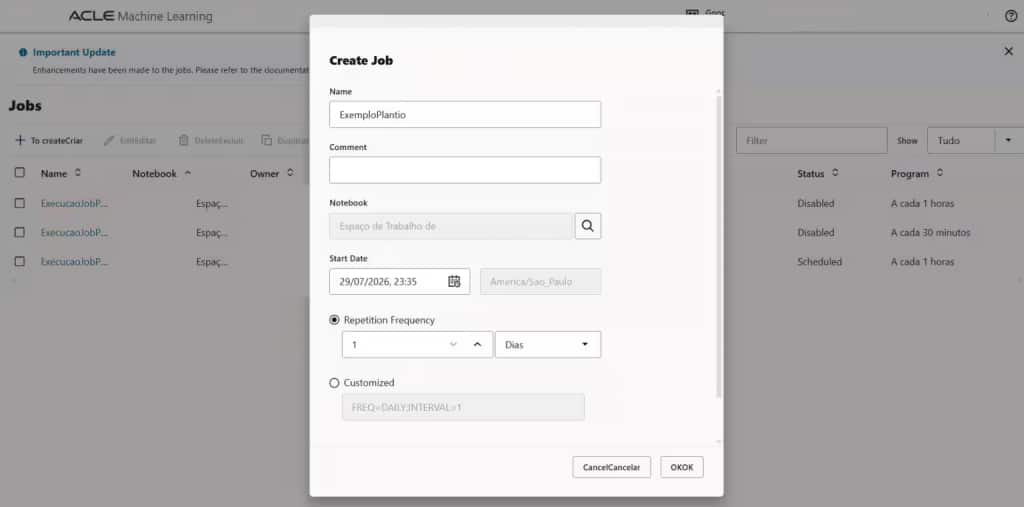
This exercise it’s very simple but let’s suppost that we have dinamic restrictions and variables, changing every day! We need the OML job. With this feature we can choose which notebook we want to execute and the exactly frequency.
Operations Research is a broad discipline with many different use cases and applications. It is not only a matter of technology, but also of applying mathematical and optimization approaches to solve complex problems. This is one possible approach for implementing a solution of this kind. There are also opportunities to leverage GPUs and artificial intelligence to further enhance the solution and deliver additional value.
Additionally, we can use Oracle APEX to build enterprise applications. Imagine being able to build an application with little to no coding to make available all the optimizations we discussed in this article. For example, this can keep parameters accessible so business users can make adjustments.
In the next article, I will explore the possibilities of using GPUs, NVIDIA libraries, and other advanced techniques to further enhance this type of solution.
Call for Action
Check out the resources below to learn more!
Learn to solve math and optimization problems using PuLP library and Python:
https://pypi.org/project/PuLP/
Try OML and develop machine learning models, using SQL, Python and R language and many other features with Oracle Machine Learning:
https://www.oracle.com/br/artificial-intelligence/database-machine-learning/
Explore Oracle APEX for building enterprise applications: