How we achieved a 4.2x GPU utilization improvement by fixing bottlenecks upstream of captioning while streaming end-to-end from OCI Object Storage.
1. Introduction
Vision-language models (for example, NVIDIA Nemotron Nano 2 VL) are often the practical choice for industrial video captioning because they maximize throughput. They batch efficiently, fit within GPU memory alongside pre/post-processing, and deliver more predictable latency – reducing tail effects that can disrupt a streaming pipeline. At scale, captioning is a per-clip cost applied millions of times, so predictable latency and resource footprint matter as much as caption quality.
In our deployment on OCI GPU Compute instances with NVIDIA H100s, the primary bottleneck was the upstream CPU data-preparation path (decode and clip assembly), not GPU inference. GPU utilization hovered around ~12% because CPU stages could not supply caption-ready clips at a steady rate. This post shows how queue behavior made the constraint visible and how targeted CPU-side changes increased utilization to ~50% while keeping the pipeline streaming end-to-end from OCI object storage.
2. Why this problem exists: multimodal data at petascale
At petascale, multimodal/video foundation models are constrained less by training than by continuous data preparation – ingest/normalize raw video, segment clips, decode frames, generate captions/embeddings, filter, and write outputs at sustained throughput. In a representative run (~100 million short-form videos on ~50 NVIDIA H100 nodes over ~35 days), any under-provisioned CPU-side stage (scene detection, transcoding, frame extraction) becomes the primary bottleneck by limiting the rate of caption-ready clips delivered to GPU inference, driving queue buildup and lower GPU utilization.
3. System overview: the streaming, composable pipeline (CPU tier + GPU tier)
We built a continuously streaming, composable pipeline for high-throughput multimodal curation that avoids using the cluster as temporary storage. It is implemented in NVIDIA NeMo Curator, using a stage-graph of discrete operators connected by bounded queues with backpressure and per-stage concurrency controls, so each step can be scaled independently. Because local disk becomes a hidden limiter at scale (capacity, fragmentation, scratch management, hard-to-debug failures), the pipeline follows an end-to-end pattern: read from OCI Object Storage, process in a streaming pipeline using primarily ephemeral in-memory buffers with minimal local disk, and write curated outputs back to OCI Object Storage; scaling on OCI Compute is then a matter of adding CPU/GPU workers and rebalancing Ray/NeMo Curator actors, not redesigning storage.
The pipeline runs as 16 concurrent stages across two resource tiers, and overall throughput is set by the slowest stage – if an upstream CPU stage lags, downstream stages (including GPU inference) are underutilized. CPU-heavy ingestion/preprocess stages include: download, remux, scene detection (our primary bottleneck), clip transcoding, motion decoding, motion filtering, frame extraction, and a custom OCR filter. Downstream stages combine additional quality filters and GPU inference: custom blur filtering, custom aesthetic filtering, Jitter filtering (some GPU-backed), InternVideo2 frame creation (CPU), InternVideo2 embedding (GPU), vLLM preparation (CPU), vLLM captioning with NVIDIA Nemotron Nano (GPU), and a final clip-writer stage streaming results back to OCI Object Storage. See Figure 1 for a visualization of the 16-staged pipeline.
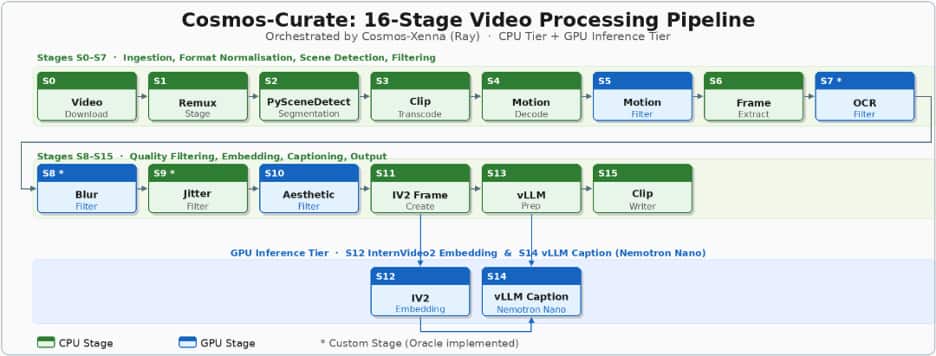
Figure 1: – Nemo Curator: 16-Stage Video Processing Pipeline
4. The symptom: Nemotron workers were idle (and the reason wasn’t Nemotron)
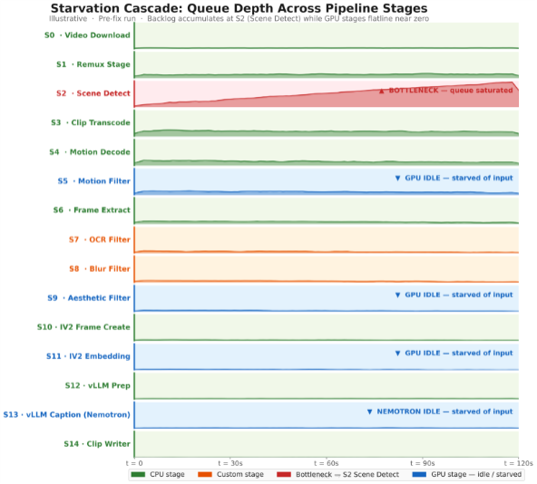
Although the vLLM caption stage (Nemotron Nano 2 VL on H100s) was GPU-accelerated, end-to-end throughput stayed below target. Cluster metrics showed ~12% GPU utilization, indicating a feed-rate bottleneck rather than slow inference. Upstream CPU stages (remuxing, scene detection, transcoding) were not producing caption-ready clips consistently, so the queues into the GPU stages repeatedly drained and the H100 workers went idle. Queue-depth timelines made this explicit: backlog built up ahead of the CPU bottleneck while queues immediately upstream of the GPU stages collapsed toward zero – showing the fix was in the CPU pipeline, not Nemotron Nano.
5. Diagnostics: how to detect starvation in a multimodal pipeline
Diagnosing starvation in a multimodal pipeline is less about profiling a single stage and more about verifying that work is flowing smoothly from ingestion to output. In practice, three signals tell you whether your GPUs are the bottlenecks, or simply waiting for upstream stages to feed them.
- The first signal is queue behavior across adjacent stages. In a healthy streaming pipeline, queues fluctuate but don’t trend toward runaway growth or persistent emptiness. Starvation shows up as a specific pattern: a queue builds up immediately before a bottleneck stage, while queues downstream collapse toward zero. If your captioning stage’s input queue is frequently empty while an earlier stage is accumulating backlog, the GPUs aren’t the problem—the pipeline is failing to deliver caption-ready clips reliably. Plotting queue depth over time per stage (even at coarse granularity) makes this visible quickly.
- The second signal is a stage-throughput mismatch. Measure each stage’s sustained throughput in the same units (e.g., clips/min or tasks/s) and compare it to the pipeline target. The end-to-end rate cannot exceed the slowest stage, so a single under-provisioned CPU stage (scene detection, remuxing, transcoding, frame extraction) can throttle everything behind it. A simple “capacity table” for each stage—workers × tasks/sec per worker—often reveals the constraint faster than code-level profiling.
- The third signal is GPU utilization that doesn’t correlate with allocated GPU capacity. If GPUs are fully allocated but utilization is low (for example, ~10–15%), you’re typically not compute-bound. Combine utilization with scheduler/worker metrics: are GPU workers spending time “idle” or “waiting for input”? If yes, the GPU stage is starved, and tuning the model won’t move the end-to-end needle until the feed rate improves.
6. The fixes: four upstream changes that unlocked Nemotron Nano throughput
We fixed the starvation cascade by targeting the CPU stages that were gating the flow of caption-ready clips into the Nemotron (vLLM) stage. Each change followed the same pattern: identify where work was piling up, confirm the root cause (under-provisioning vs. inefficient execution), then rebalance concurrency so the downstream GPU stages stayed fed.
Fix #1: Clip transcoding queue buildup (starvation risk).
- What we saw: The ClipTranscoding stage’s input queue frequently grew while downstream stages—especially GPU stages—were intermittently idle.
- Root cause: The stage was simply under-provisioned relative to the rate of incoming clips.
- Fix: We tuned Ray actor counts and CPU allocations for transcoding to increase effective parallelism.
- Impact: The input queue drained to near-zero and the rest of the pipeline received a steadier stream of clips, reducing idle time in downstream workers.
Fix #2: Single-threaded FFmpeg decoding/encoding on H100 nodes.
- What we saw: even after adding actors, transcoding throughput per actor was lower than expected for the available CPU resources.
- Root cause: One of the design choices in H100/A100 architecture is the absence of any NVENC encoder (done to maximize die space for AI compute). Consequently, video encoding is forced entirely onto the CPU using software encoders like libopenh264. If FFmpeg is not explicitly configured to parallelize this workload, it defaults to single-threaded execution. This turned our transcoding stage into a hidden, severe bottleneck, leaving the majority of our CPU cores sitting idle and simultaneously starving our downstream GPU-heavy stages of data.
- Fix: We updated the implementation and FFmpeg parameters to use multi-threaded CPU transcoding (using the —threads parameter) mapping the thread count to the dedicated CPU allocation for each Ray actor.
- Impact: throughput per actor improved by ~55% (from 0.09 → 0.14 tasks/s), which eliminated the transcoding backlog and materially improved the feed rate into downstream stages.
Fix #3: Remux stage resource allocation.
- What we saw: The pipeline backed up near the very beginning while normalizing heterogeneous source formats into a consistent MP4 stream.
- Root cause: Insufficient concurrency in the Remux stage relative to the input volume.
- Fix: We increased the number of Ray actors (roughly one actor per node) to keep pace with ingestion.
- Impact: We removed a front-of-pipeline throttle that was limiting overall intake and causing periodic downstream starvation.
Fix #4: PySceneDetect saturation (the primary bottleneck).
- What we saw: PySceneDetect workers were fully saturated – input queue growing continuously while all downstream stages, including Nemotron captioning, were starved of work.
- Root cause: Scene detection is computationally heavy (mathematically calculating pixel differences across frames), and the initial worker allocation was insufficient for the target throughput.
- Fix: We scaled horizontally by increasing the Ray Actor count for PySceneDetect stage from 1 to 8 workers per node, raising its throughput ceiling to match pipeline demand. We also evaluated Ray’s native autoscaling for this stage and empirically verified that our static 8-worker configuration performed on par with the dynamically autoscaled numbers.
- Impact: Queue depth normalized, downstream GPU stages returned to high utilization, and overall video processing rate tripled.
Fix #5: Using Low-Resolution Proxies for Scene Detection Instead of High-Res Sources
- What we saw: The PySceneDetect stage was heavily bottlenecked, consuming a massive amount of CPU time per video and acting as a major roadblock in the pipeline.
- Root cause: Our source videos were high-resolution 4K(2160×4096). PySceneDetect stage relies on OpenCV to perform pixel-by-pixel mathematical comparisons across consecutive frames to find scene cuts. Processing raw 4K required the CPU to analyze roughly 8 million pixels per frame, creating a heavy computational load.
- The Fix: While PySceneDetect’s underlying FFmpeg integration can downscale video on the fly, we found that explicitly separating this step yielded better performance. Before scene detection, we introduced an FFmpeg subprocess to downscale the 4K video into a 360p proxy file. We wrote this proxy directly to fast local NVMe storage, and pointed PySceneDetect at the proxy instead of the 4K source.
- Impact: Explicit downscaling with NVMe writes outperformed on-the-fly conversion, boosting PySceneDetect throughput by 17%.
7. Nemotron Nano 2 VL before/after: utilization and throughput results
After rebalancing the upstream CPU stages, the effect on the Nemotron Nano captioning stage was immediate and measurable. The headline improvements were:
| Metric | Before | After | Notes |
| H100 GPU utilization (captioning workers) | ~12% | ~50% | Utilization increased primarily by eliminating upstream starvation |
| Throughput | ~50 videos per GPU hour | ~150 videos per GPU hour | Videos are shortform ~30 seconds each |
| End-to-end impact | — | ~3× throughput gain | Observed in benchmark tests; validated further on larger-scale runs |
It’s worth noting that 100% utilization is not a realistic goal in a real streaming pipeline. This pipeline mixes CPU and GPU stages, dealing with variable media properties (bitrate, codec, resolution), and relying on queues/backpressure to keep the system stable under bursts and stragglers. Moving from ~12% to ~50% utilization is often the difference between a pipeline that struggles to finish and one that can run reliably at production scale avoiding idle time.
8. Caption quality at scale: Nemotron Nano vs A Similarly Sized Model
We ran a targeted caption quality evaluation comparing Nemotron-Nano-12B-v2-VL against a similarly sized model, using a methodology that scales even when human reference captions aren’t available.
Because our video segments did not come with ground-truth captions, we constructed a proxy reference set by generating three independent GPT-4o captions per segment. We then compared each model’s captions against these references using a mix of semantic and lexical metrics—Sentence-T5 cosine similarity (semantic alignment), BERTScore (token-level similarity using contextual embeddings), and an LLM-based 10-point Likert score from GPT-4o intended to approximate a human “how good is this caption?” judgment. Since the references were model-generated rather than human-authored, we treat these results as comparative rather than absolute.
| Model | Sentence-T5 cosine | BERTScore | GPT 10-point Likert scale |
| Nemotron-Nano-12B-v2-VL (GA container) | 0.87 | 0.28 | 6.53 |
| Similarly Sized Model | 0.86 | 0.19 | 6.38 |
Overall, Nemotron Nano performed on par with, or slightly ahead of, Similarly Sized Model on the metrics that emphasize meaning and readability. Nemotron achieved slightly higher Sentence-T5 cosine and a higher Likert score, suggesting comparable or better semantic fidelity and “human-likeness.” It also produced a higher BERTScore, indicating closer lexical alignment to the reference captions.
The practical takeaway is simple: both models produced coherent, relevant captions, and Nemotron Nano 2 VL’s quality was competitive while delivering the throughput characteristics we needed for large-scale processing. Given that captioning is applied to every clip, that combination—strong-enough quality with predictable, high throughput—made Nemotron Nano 2 VL the right fit for our pipeline.
9. Conclusion: the broader principle
At this scale, the headline lesson is simple: NVIDIA Nemotron Nano 2 VL can caption at very high throughput on H100s, but the model is only as fast as the pipeline that feeds it. If upstream CPU stages can’t keep up, the most capable GPU inference stack will still sit idle—and you’ll pay for it in both schedule and cost.
What made the difference for us was treating the system end-to-end: a streaming design that moves data from Object Storage → pipeline → Object Storage without relying on local cluster disks, stage-level observability that made starvation visible, and targeted tuning of CPU-heavy stages so they could reliably supply work to the GPU tier. That combination is what turned low utilization into sustained throughput and made processing at the scale of hundreds of petabytes practical in our environment. On Oracle Cloud Infrastructure, pairing OCI Object Storage with OCI Compute (NVIDIA H100 GPUs) let us keep data streaming end-to-end while tuning CPU stages to fully utilize the GPU tier.
We would like to acknowledge the OCI AI Foundations team members Pradipta De, Ranjeet Gupta, Sujeeth Bharadwaj, and Graham Horwood for their contributions to this blog.