In today’s data-driven world, the necessity for scalable resources in model deployment is paramount across various industries. The capability to dynamically adjust computing resources in response to fluctuating demands isn’t just a convenience, but a critical component for maintaining efficiency and cost-effectiveness. This adaptability is particularly vital in fields where data volumes and processing needs can change unpredictably. The concept of autoscaling becomes especially relevant in such scenarios, allowing for real-time adjustment of resources to meet the varying demands of data processing and analysis. When we turn our focus to financial institutions, the importance of autoscaling becomes even more pronounced. Financial sectors are characterized by their fast-paced environments and the need to process vast, complex datasets.
Here, the implementation of autoscaling in Oracle Cloud Infrastructure (OCI) Data Science for model deployment becomes crucial. Imagine a large retail bank that has recently deployed a sophisticated AI model to predict loan defaults and analyze customer creditworthiness. This model, integral to the bank’s loan approval process, operates on vast amounts of data, including transaction histories, customer interactions, and market trends. Initially, the model is deployed on a fixed OCI resource allocation, but soon, the bank faces the following challenges:
- Varying load during financial cycles: The bank experiences peak load times during the end of financial quarters when many businesses apply for loans. During these times, the model needs to process a high volume of requests, leading to potential slowdowns or even service downtime.
- Unpredictable market events: Sudden market events, such as economic downturns or policy changes, can trigger a surge in customer inquiries and transactions, demanding immediate scaling of resources to maintain performance.
- Cost optimization: During off-peak hours or days with low customer interaction, the bank’s AI model consumes resources that aren’t efficiently utilized, leading to unnecessary expenditure
To deal with these challenges, you simply enable autoscaling in your deployment and then you select the desired scaling metrics and thresholds, and Model Deployment Auto Scaling will do the rest, reading metrics from your deployment and triggering the scaling operation whenever needed. In this blog post, we demonstrate on how autoscaling feature can be configured for Oracle Cloud Infrastructure (OCI) Data Science model deployments to handle increased or decreased loads.
Autoscaling Overview and Key Features
The essence of the autoscaling solution revolves around establishing rules based on the metrics emitted by the model deployment. It involves augmenting compute power when metrics surpass a predefined utilization threshold, referred to as scaling out, and reducing compute power when metrics fall below a specific utilization value, known as scaling in. When scaling is required for CPU utilization, virtual machine (VM) instances can be added or removed from the deployment to fine-tune processing power. Adding an instance alleviates the processing load on existing instances, and this form of scaling is termed horizontal scaling. It involves the incorporation of additional instances with the same VM shape into the deployment.
In the context of autoscaling, the model deployment ensures zero downtime for serving inference requests. The old instance keeps service inference requests when the new ones are getting added, ensuring a seamless transition without interruptions. Autoscaling in OCI Data Science Model Deployment includes the following key features:
- Dynamic Resource Adjustment: Autoscaling automatically increases or decreases the number of compute resources based on real-time demand (for example, autoscale and downscale from 1 to 10), ensuring that the deployed model can handle varying loads efficiently.
- Cost Efficiency: By adjusting resources dynamically, autoscaling ensures you only use (and pay for) the resources you need. This can result in cost savings compared to static deployments.
- Enhanced Availability: Paired with a load balancer, autoscaling ensures that if one instance fails, traffic can be rerouted to healthy instances, ensuring uninterrupted service.
- Customizable Triggers: Users can completely customize the autoscaling query using MQL expressions (Monitoring query Language Expressions).
- Load Balancer Compatibility: Autoscaling works hand-in-hand with load balancers where LB bandwidth can be scaled automatically to support higher traffic, ensuring optimal performance and reducing bottlenecks.
- Cool-down Periods: After scaling actions, there can be a defined cool-down period during which the auto scaler won’t take further actions. This prevents excessive scaling actions in a short time frame.

Model Deployment Autoscaling in Action
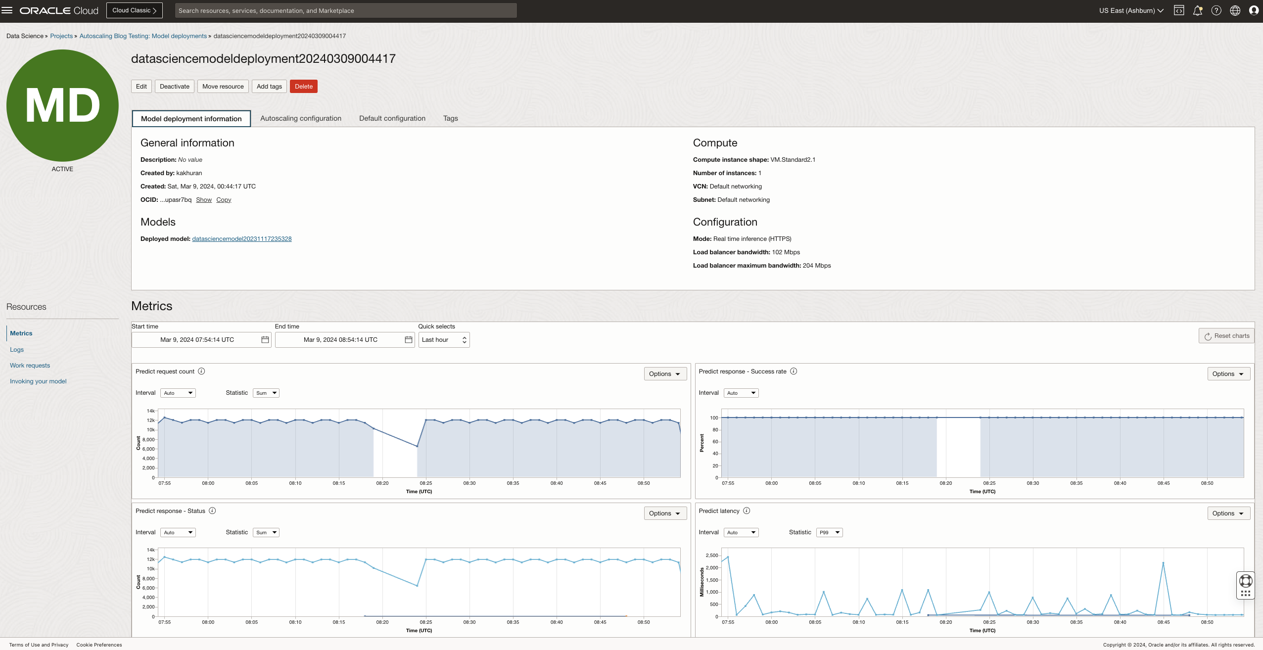
You can proceed to the Oracle Cloud Infrastructure (OCI) Data Science console and navigate to the “Model Deployments” section. Here, they have the flexibility to either create a new model deployment or select an existing one to enable autoscaling. To demonstrate autoscaling, we use an existing model deployment resource configured with a small-size model and hosted on a single VM. Setting up autoscaling involves identifying the right set of policies and applying those scaling policies. For more details on various options refer to the Configuring autoscaling in Model Deployments . The following figure shows the model deployment resource that is already created:

Understanding Application Characteristics
To derive the right scaling policy, we first determine the application characteristics with the chosen instance type. But before that, understanding the metrics that the Model Deployment emits is important. At a high level, these metrics are categorized into three classes: invocation metrics, latency metrics, and utilization metrics. To learn about different metrics, refer to this Model Deployment Metrics Public documentation.

Examine your chosen infrastructure’s utilization metrics to identify the bottlenecks in the system, if any. For CPU instances, the bottleneck can be in the CPU or memory, while for GPU instances, the bottleneck can be in GPU utilization and its memory.
![]() .
. 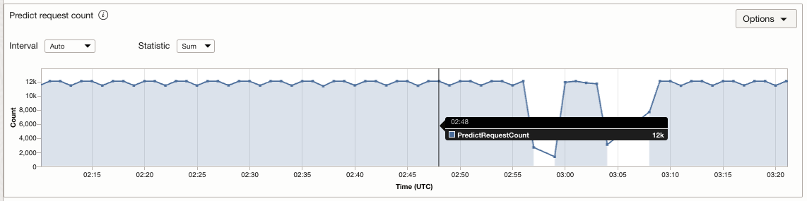
Let’s try correlating the CPU utilization with the request per min (RPM) to understand the impact of high or low request load on the application. In many cases, when the load is high and the CPU is saturated, the deployment can no longer handle any more requests and performance begins to deteriorate. The following graph shows that when the RPM spikes, the CPU utilization reaches almost 100% and the predict latency also becomes higher. However, when the RPM drops, the utilization hovers around 20% or minimum.

Defining Thresholds
To define the thresholds, we need to understand the request pattern for the application. We want to know the maximum and minimum number of requests that we can expect to receive for our application. This range helps us understand how the CPU utilization looks for our RPM bounds using that we can derive thresholds for the scaling policy. For this example, the maximum requests per minute (max) is approximately 15K, and the minimum request per minute (min) is approximately 9K. We can see that CPU utilization stays between 45–65% for this range, and the average is 55%.
When the new instance is added after scaling, requests start getting evenly distributed but the CPU utilization is not exactly halved. There is some baseline CPU utilization on every instance even when no prediction requests are coming, which should be considered for calculating our scaling policy thresholds. The scale-out threshold can be your maximum CPU utilization but the scale-in threshold should be less than X, where X can be calculated using the formula:
CPU utilization without any load + (maximum CPU utilization - CPU utilization without any load)/2
This ensures we are not scaling in again after a scale-out action has just been performed.
Another consideration that you should make when deciding thresholds is whether you want to optimize for cost or availability. By keeping a wider range for threshold (scale_in, scale_out) you opt for availability, whereas narrow for cost. We decided to keep our thresholds at (30, 65) preferring availability over cost, but you are free to choose any scale-in threshold value as long as it is less than X. The request pattern load can also help us predetermine how many instances would be needed for our application. You can calculate the maximum number of instances using:
floor(maximum RPM expected/ mean RPM)
Enable Autoscaling
Before we start updating a model deployment to enable autoscaling, we need to add a policy to give the autoscaling system access to read metrics from the tenancy, where these metrics are posted.
allow service autoscaling to read metrics in tenancy where target.metrics.namespace='oci_datascience_modeldeploy'

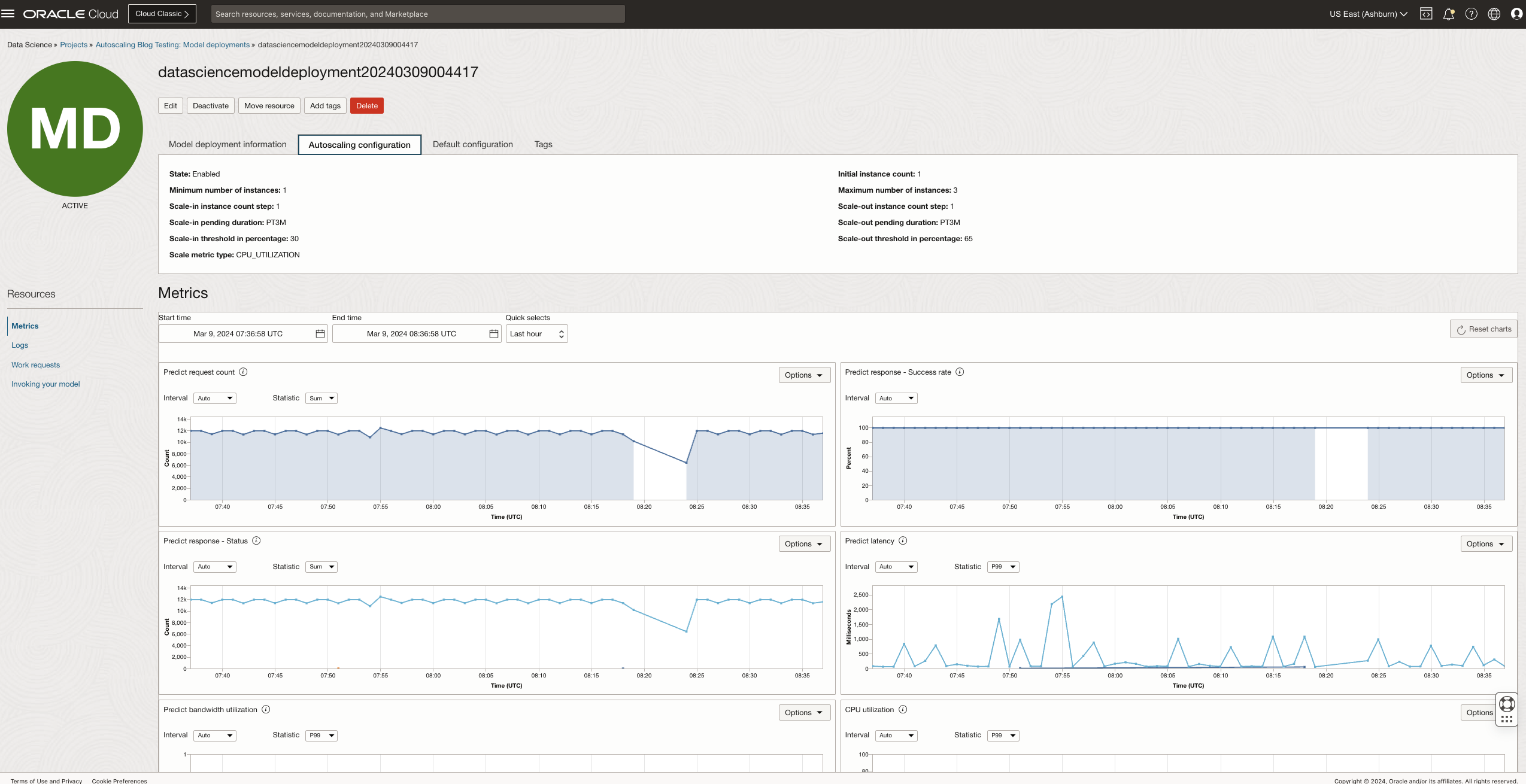
Once the above policy is submitted, users can start setting up autoscaling on the model deployment resource. Both the Compute and Load Balancer autoscaling can be configured. Next, we click on the Edit button to enable autoscaling and Select the checkbox that says “Enable autoscaling“.

A new panel will open with field values pre-populated. You can modify the values as per your needs. By default, the autoscaling will be enabled using the CPU Utilization metric. We updated thresholds to – scale out at 65% and the scale in at 30%.

Optionally, if you want to autoscale the LB bandwidth, go to Show advanced options and provide a value for the maximum bandwidth. Note that, the maximum bandwidth should be greater than the minimum and less than or equal to twice the minimum bandwidth.

Finally, click the Submit button and await the activation of the model deployment. When active, the deployment instance is equipped with the autoscaling feature.
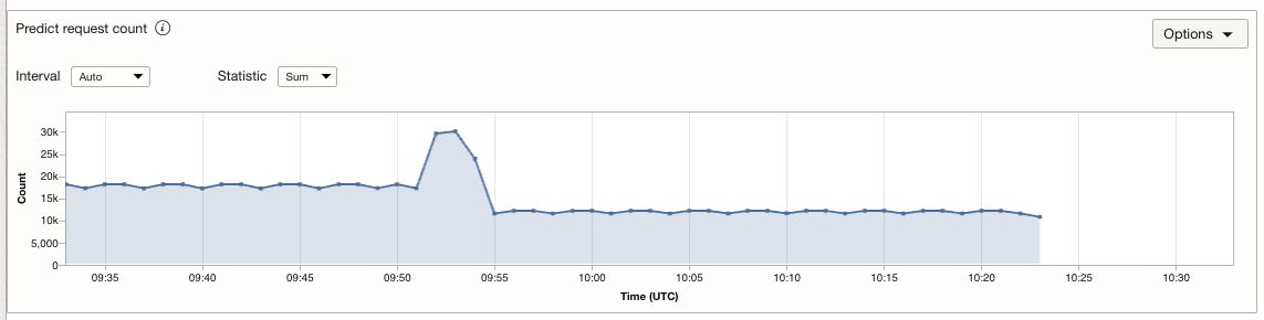
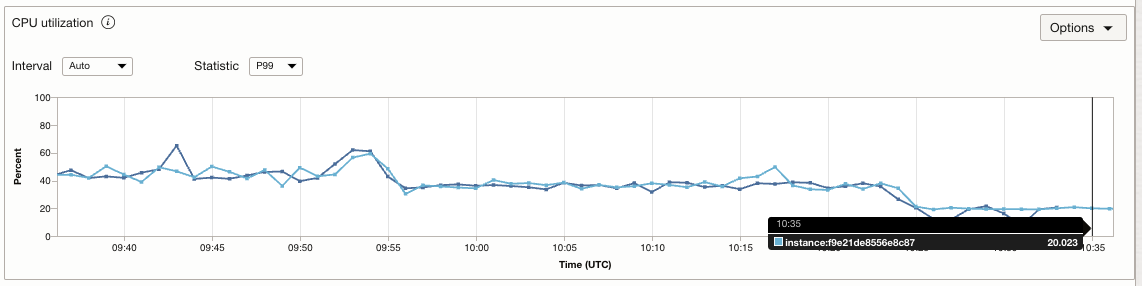
Watch the instance for the activation of scaling conditions. As the influx of requests rises, CPU utilization also increases. You can notice the start of the scaling operation when CPU utilization surpasses the preset threshold of 65%. Upon the completion of the scaling operation, the workload is evenly distributed across all available instances. This distribution leads to a decrease in CPU utilization and an enhancement in the application’s availability.The following figure shows the CPU utilization per instance, before and after scaling

Throughout the scaling process, you can monitor work request logs, providing updates on the progress. These logs detail the operations being conducted, as well as the previous and updated sizes of the deployment.

When the requests stop coming or RPM reduces to a level where the scale-in threshold of 30% is breached, a scale-in operation is triggered, hence saving cost.
 .
. 
Advanced Scaling Conditions
You can also select a custom scaling metric type, where users can write their own MQL queries to configure autoscaling. This feature allows for the creation of more sophisticated queries, including the ability to combine multiple queries using operators like “AND” and “OR”, employ various aggregation functions, and choose a specific evaluation window. Utilizing this option provides greater control over the scaling conditions, enabling a more customized and precise setup tailored to specific needs.
For example, a customer knows about the request pattern and its impact on resource utilization. Instead of choosing CPU utilization as the metric, the customer selects the Predict Request Count metric directly. From the previous analysis, we know that the maximum RPM was 15K, for which the maximum CPU utilization was 65%. So, instead of using 65 as the CPU utilization threshold, we use 15K for the predict request count scale-out threshold. Similarly, we select 9K for the scale-in threshold. Our scaling queries become:
Scale-out:
PredictRequestCount[1m]{resourceId = "MODEL_DEPLOYMENT_OCID"}.grouping().sum() > 15000 |
Scale in:
PredictRequestCount[1m]{resourceId = "MODEL_DEPLOYMENT_OCID"}.grouping().absent() == 1 || PredictRequestCount[1m]{resourceId = "MODEL_DEPLOYMENT_OCID"}.grouping().sum() < 9000 |
To select this option, just select Scaling Metric type Custom in Console and insert these queries in the fields for scale-out and scale-in custom metric query.

For more details on how to use Custom metrics, you can refer to Documentation on Custom Metrics.
Understanding Constraints and Best Practices
- Users can Enable/Disable both autoscaling on Instances and LB Bandwidth for Model Deployment resources.
- There is a minimum cool-down period of 10 minutes between each scaling event that is enforced.
- We support Threshold Based Autoscaling Policy. Users cannot provide more than one policy.
- Scaling logs will be exposed through work request logs updated on each scaling action.
- Users can enable LB autoscaling by setting maximum BW along with minimum BW value. The maximum will be restricted to twice the minimum.
- Users can only use metrics that are provided by the service to set up autoscaling rules.
- The same instance count restrictions apply with autoscaling (the maximum count supported is 10).
Conclusion
In conclusion, the implementation of autoscaling in Oracle Cloud Infrastructure (OCI) stands as a transformative solution, particularly for financial institutions like our example retail bank. By utilizing dynamic and intelligent scaling of resources, the bank significantly enhances the performance and reliability of its AI model for credit assessment while achieving substantial cost efficiency. Autoscaling adeptly ensures the bank’s ability to handle unpredictable workloads, from market fluctuations to seasonal trends, thus maintaining high service availability and customer satisfaction. Looking towards the near future, autoscaling is poised to evolve further by supporting GPU shapes, an advancement that will be particularly beneficial for handling Large Language Models (LLMs). This capability will open new avenues for financial institutions to leverage more complex and resource-intensive AI models, further enhancing their analytical and predictive capacities. In the ever-changing digital financial landscape, this technology is not merely a strategic tool for resource management; it is a vital component in fostering agility and resilience in financial institutions. With the adoption of autoscaling in OCI, these institutions are well-equipped to ensure their technological infrastructure remains as adaptive and forward-thinking as their financial strategies.
Try Oracle Cloud Free Trial for yourself! A 30-day trial with US$300 in free credits gives you access to OCI Data Science service. For more information, see the following resources:
- Documentation Model Deployment Documentation
- Full sample including all files in OCI Data Science sample repository on Github.
- Visit our OCI Data Science service documentation.
- Configure your OCI tenancy with these setup instructions and start using OCI Data Science.
- Star and clone our new GitHub repo! We included notebook tutorials and code samples.
- Watch our tutorials on our YouTube playlist
- Try one of our LiveLabs. Search for “data science.”