Introduction
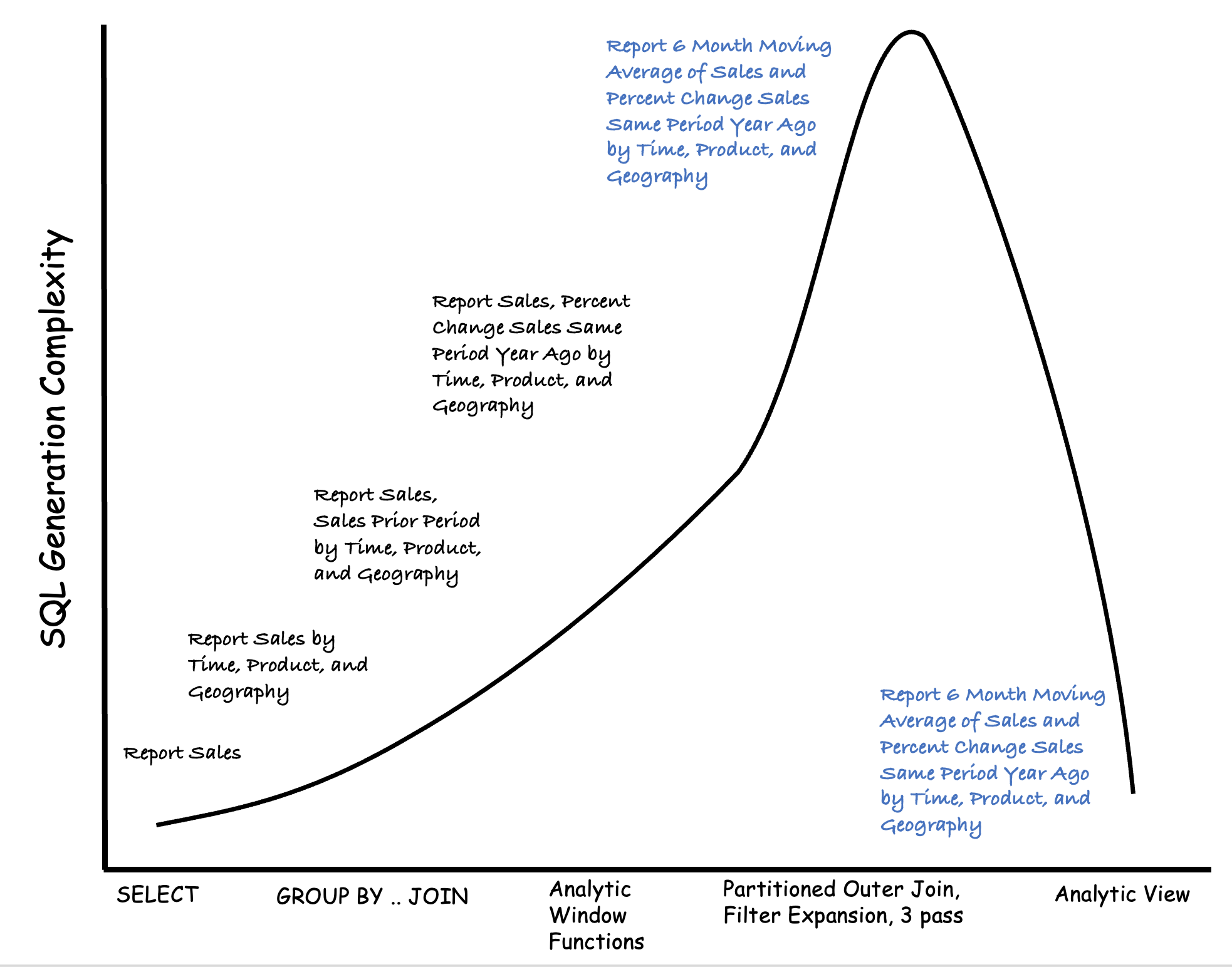
Writing or generating queries can be difficult, especially when queries must return analytic calculations at aggregate levels. For example, writing a single query that returns a measure, such as a percent change in sales for the current month compared to the same month last year, is challenging. It is a three-pass query, with aggregation, partitioned outer joins, filter expansion on the first pass, analytic window functions on the second pass, and some basic math on the final pass.
People typically do not write these queries themselves. It is just too hard. They use business intelligence tools like Oracle Analytic Cloud (OAC) instead. OAC has nice data visualizations, but the hard work is done in the OAC server – generating the queries.
The developer is on the hook for SQL generation when writing a custom application, for example, using Oracle Application Express (APEX). Writing a single analytic query that services a report or graph can be complex. Writing a SQL generator that supports data selections, different aggregations, changing dimensionality, and various parameterized calculations is more complicated. It is something the typical developer might not attempt.
Why is it so hard? It is hard because the developer needs to do all the work. The developer must write a SQL generator and manage the metadata to support it. Tables are great at storing and retrieving data, but tables do not write the queries. Do they?
What if there was a table that did write the query? What if that table came with a semantic model? What if that table supported special functions that made expressing analytic calculations easy? And what if an application could query that table with simple, template-like SELECT statements? A developer could write powerful custom applications in no time!
There is such a table, but it is not a table. It is an Oracle Analytic View.
Some developers might fear that analytic views are complicated. That there is a steep learning curve. Do not worry. Creating an analytic view is not much more complicated than writing a SQL query that joins tables and aggregates data. A little learning and additional work upfront will pay significant dividends in the form of simplified queries and the ability to add rich analytic content to applications.
About Analytic Views
Oracle Analytic Views are a feature of the Oracle Database that lets developers define relationships between data and calculate various aggregations and calculations. Analytic views make it easier for users to analyze large amounts of data and perform complex analytical queries.
Analytic views simplify the process of building complex analytical queries by providing a pre-built view of the data that is queried using familiar SQL constructs. By using analytic views, developers can reduce the time and effort required to write complex SQL queries and improve the performance of their queries by pre-calculating and caching the results of commonly used aggregations.
An analytic view uses a dimensional model to organize one or more dimension tables with a fact table. Analytic views support various analytic and aggregation functions including time series, ranking, hierarchical shares (ratios).
Run This Post as a Live SQL Tutorial
All of the examples (and more) in this post can be run in two Oracle Live SQL tutorials:
- Analytic View Quick Start Part 1 – Easy Analytic View DDL Statements
- Analytic View Quick Start Part 2 – Simple Query Templates for Developers
There are many more analytic view tutorials on Live SQL.
Creating Analytic Views, Simply
An analytic view can be designed with only the necessary structural elements and no descriptive metadata, or it may include complex structures and rich metadata.
A simple analytic view will have all the elements necessary to support analytic calculations and straightforward, reusable query templates. Designing this analytic view is no more difficult than writing a query that joins tables in a star schema and aggregates data using GROUP BY.
Examples in this post show the minimal DDL needed to create an analytic view using the sample data in the AV schema in Oracle Live SQL. The Data Studio Analysis application in the Oracle Autonomous Database can be used to create the same analytic view without coding.
A Traditional View
It might be useful to use the following query as a baseline.
SELECT
    t.year_name
  , p.department_name
  , g.region_name
  , SUM(f.units)
  , SUM(f.sales)
FROM
    av.time_dim      t
  , av.product_dim   p
  , av.geography_dim g
  , av.sales_fact    f
WHERE
        t.month_name = f.month_id
    AND p.category_id = f.category_id
    AND g.state_province_id = f.state_province_id
GROUP BY
    t.year_name
  , p.department_name
  , g.region_name
ORDER BY
    t.year_name
  , p.department_name
  , g.region_name;
What is this view doing? It is:
- Selecting a list of columns where some columns are playing the role of measures. Let’s say the YEAR_NAME, DEPARTMENT_NAME, and GEOGRPAHY_NAME columns are playing the role of attributes.
- Aggregating the measures.
- Selecting from tables, which are joined.
- Sorting rows.
An Analytic View
A simple analytic view can do the same things, plus three additional things, very easily:
- Define aggregation and navigation paths in hierarchies.
- Support calculating measures using analytic view expressions.
- Provide a set of hierarchical columns that simplify query generation.
Analytic views are a system of objects: attribute dimensions, hierarchy views, and the analytic view. Each allows for reusability. Attribute dimensions include most of the metadata used by hierarchies. More than one hierarchy can be created from an attribute dimension. Analytic views reference hierarchies. More than one analytic view can reference a single hierarchy. This reusability can save much work.
Run the Live SQL Tutorial for more details. The most important topics are covered in this post.
Attribute Dimension
The attribute dimension lists columns in the ATTRIBUTES clause and includes a list of levels. Each level has a KEY column. Levels can have an ORDER BY column used for sorting. In cases where the level KEY is not a good label (for example, ID columns with integers) a different column is used as the MEMBER NAME. The DETERMINES clause states that for each level KEY value, there is only one value of the determined attribute. The DETERMINES clause enable many SQL optimizations.
Just like tables have many properties that default if not set in a CREATE TABLE statement, so do attribute dimensions. To see all the defaulted values, get the DDL after creating the attribute dimension using a simple DDL statement
The following statement creates the attribute dimension used with the TIME_DIM table.
CREATE OR REPLACE ATTRIBUTE DIMENSION time_attr_dim
USING av.time_dim
ATTRIBUTES
 -- List of columss
 (year_name,
  quarter_name,
  month_name,
  month_end_date)
-- A level of aggregation
LEVEL year
  -- The primary key of the level
  KEY year_name
LEVEL quarter
  KEY quarter_name
  -- For each value of QUARTER_NAME, there is only one value of YEAR_NAME
  DETERMINES (
    year_name)
LEVEL month
  KEY month_name
  -- Sort months by MONTH_END_DATE
  ORDER BY month_end_date
  DETERMINES (
    month_end_date,
    quarter_name);
Hierarchy View
The hierarchy view is simple, just a list of levels organized as child-parent relationships.
CREATE OR REPLACE HIERARCHY time_hier
USING time_attr_dim
 (month CHILD OF
  quarter CHILD OF
  year);
Simple!
Additional Attribute Dimensions and Hierarchy Views
The attribute dimensions and hierarchies for product and geography follow the same pattern.
CREATE OR REPLACE ATTRIBUTE DIMENSION product_attr_dim
USING av.product_dim
ATTRIBUTES
 (department_name,
  category_name,
  category_id)
LEVEL department
  KEY department_name
LEVEL category
  KEY category_id
  MEMBER NAME category_name
  DETERMINES (
    department_name);

CREATE OR REPLACE HIERARCHY product_hier
USING product_attr_dim
 (category CHILD OF
  department);

CREATE OR REPLACE ATTRIBUTE DIMENSION geography_attr_dim
USING av.geography_dim
ATTRIBUTES
 (region_name
  , country_name
  , state_province_name
  , state_province_id)
LEVEL region
  KEY region_name
LEVEL country
  KEY country_name
  DETERMINES (
    region_name)
LEVEL state_province
  KEY state_province_id
  MEMBER NAME state_province_name
  DETERMINES (
    country_name);

CREATE OR REPLACE HIERARCHY geography_hier
USING geography_attr_dim
 (state_province CHILD OF
  country CHILD OF
  region);
The Analytic View
The analytic view identifies FACT measures from the SALES_FACT table and joins the fact table to hierarchies using the REFERENCES clause. FACT measures include aggregation operators. SALES_PRIOR_PERIOD is an example of a calculated measure.
CREATE OR REPLACE ANALYTIC VIEW sales_av
USING av.sales_fact
DIMENSION BY
  (time_attr_dim
    KEY month_id REFERENCES month_name
    HIERARCHIES (
      time_hier DEFAULT),
   product_attr_dim
    KEY category_id REFERENCES category_id
    HIERARCHIES (
      product_hier DEFAULT),
   geography_attr_dim
    KEY state_province_id
    REFERENCES state_province_id
    HIERARCHIES (
      geography_hier DEFAULT)
   )
MEASURES
 (sales FACT sales,
  units FACT units,
  sales_prior_period AS (LAG(SALES) OVER (HIERARCHY time_hier OFFSET 1))
  );
That is all there is to it. Read on and see what this analytic view can do for you.
Getting Started with SQL
Nobody writes a complete, multi-pass analytic query as their very first SQL query. The first query is likely simple, for example, SELECT * FROM SALES_ORDERS. With experience, queries become more complex, perhaps adding GROUP BY and joins. Experienced developers might write that complex analytic query using outter joins and analytic window functions.
Follow the same pattern with an analytic view. Begin with a simple model and focus on the structure of the model. Take advantage of more advanced features as needed, with additional experience.
A simple analytic view is very powerful. It can be queried with a simple query template and can include calculated measures. It will flatten the query complexity curve on day one.
Example: Simple Aggregation
This first example is simple. The query aggregates data to the Year, Region, and Department levels.
Table Query
The following query selects directly from tables. The query follows the predictable SELECT … FROM .. WHERE … GROUP BY … ORDER BY pattern.
SELECT
    t.year_name
  , p.department_name
  , g.region_name
  , SUM(sales)
FROM
    av.time_dim      t
  , av.product_dim   p
  , av.geography_dim g
  , av.sales_fact    f
WHERE
        t.month_name = f.month_id
    AND p.category_id = f.category_id
    AND g.state_province_id = f.state_province_id
GROUP BY
    t.year_name
  , p.department_name
  , g.region_name
ORDER BY
    t.year_name
  , p.department_name
  , g.region_name;
Analytic View Queries
A query selecting from an analytic view looks similar to the query of the tables. The main difference is that the HIERARCHIES clause replaces the joins and GROUP BY.
Using Attributes
This form of the query selects attributes, which are the original colums from the tables. The analytic view can return data at any level of aggregation, so the WHERE clause uses LEVEL_NAME filters.
SELECT
    year_name
  , department_name
  , region_name
  , sales
FROM
    sales_av HIERARCHIES (
      time_hier
    , product_hier
    , geography_hier
    )
WHERE
    time_hier.level_name = 'YEAR'
    AND product_hier.level_name = 'DEPARTMENT'
    AND geography_hier.level_name = 'REGION'
ORDER BY
    year_name
  , department_name
  , region_name;
Selecting from attributes may feel familiar, but this query shares a complication with queries that SELECT from tables – the column names need to change as the levels of aggregation change. For example, many the column names would be changed if the query were to select at the Quarter, Brand, and Country levels. A SQL generator needs to handle that.
Using Hierarchical Columns
Queries that SELECT from analytic views can use hierarchical columns. These columns are part of every hierarchy and analytic view. The hierarchical columns return data at every level of aggregation, eliminating the need to navigate different columns representing different levels of aggregation. A SQL generator can be hard-coded to these columns.
The MEMBER_NAME column typically returns the hierarchy member’s descriptive name (which might differ from a KEY value). The HIER_ORDER column returns the sort order. Because both columns exist in every hierarchy, the column names are qualified by hierarchy names.
SELECT
    time_hier.member_name AS time
  , product_hier.member_name AS product
  , geography_hier.member_name AS geography
  , sales
FROM sales_av
    HIERARCHIES (
        time_hier
        , product_hier
        , geography_hier
        )
WHERE
    time_hier.level_name = 'YEAR'
    AND product_hier.level_name = 'DEPARTMENT'
    AND geography_hier.level_name = 'REGION'
ORDER BY
    time_hier.hier_order
    , product_hier.hier_order
    , geography_hier.hier_order;
Change Level of Aggregation
To change this query to select from Quarter, Brand, and Country data, change the level filters. No other changes are needed.
SELECT
    time_hier.member_name AS time
  , product_hier.member_name AS product
  , geography_hier.member_name AS geography
  , sales
FROM sales_av
    HIERARCHIES (
        time_hier
        , product_hier
        , geography_hier
        )
WHERE
    time_hier.level_name = 'QUARTER'
    AND product_hier.level_name = 'BRAND'
    AND geography_hier.level_name = 'COUNTRY
ORDER BY
    time_hier.hier_order
  , product_hier.hier_order
  , geography_hier.hier_order;
Prior Period Queries
Next, let’s add a calculation to the query: Sales Prior Period,
Table Query
The table query will need two passes. The first aggregates sales data, and the second calculates the prior periods. The partitioned outer join handles the case where data for a prior period is missing. The query should return NULL for a prior period when there is no row in the fact table.
WITH sum_sales AS (
    -- First pass, aggregate data.
    SELECT
        t.year_name
      , p.department_name
      , g.region_name
      , SUM(sales) AS sales
    FROM
        av.time_dim      t
      , av.product_dim   p
      , av.geography_dim g
      , av.sales_fact    f
    WHERE
            t.month_name = f.month_id
        AND p.category_id = f.category_id
        AND g.state_province_id = f.state_province_id
    GROUP BY
        t.year_name
      , p.department_name
      , g.region_name
),
  -- Get time periods.
  year_dim AS (
    SELECT DISTINCT
        year_name
    FROM
        av.time_dim
)
-- Second pass, calculate sale prior period.
SELECT
    b.year_name
  , a.department_name
  , a.region_name
  , a.sales
  , LAG(a.sales)
      OVER(PARTITION BY a.department_name, a.region_name
           ORDER BY
               b.year_name ASC
    ) AS sales_prior_period
FROM
    sum_sales a
    PARTITION BY ( a.department_name
                 , a.region_name ) RIGHT OUTER JOIN (
        SELECT DISTINCT
            b.year_name
        FROM
            av.time_dim b
    )         b ON ( a.year_name = b.year_name )
ORDER BY
    year_name
  , department_name
  , region_name;
Analytic View Query
The analytic view query will receive one modification and one addition, a calculated measure.
Because the calculated measure changes the definition of the analytic view for the duration of the query, this query uses the ANALYTIC VIEW USING form of the FROM clause. Add a calculated measure using the ADD MEASURES clause. Otherwise, it is the same query template as the first analytic view query.
This form of query can be used for all queries. ADD MEASURES must have at least one measure. The ROW_COUNT measure is a useful measure to include in the query template. This measure returns a constant of 1 for each row and aggregates it using SUM. It provides the row count of the query. The measure does not need to be included the SELECT list.
SELECT
    time_hier.member_name AS time
  , product_hier.member_name AS product
  , geography_hier.member_name AS geography
  , sales
  , sales_pp
FROM ANALYTIC VIEW (
    USING sales_av HIERARCHIES (
      time_hier
    , product_hier
    , geography_hier
    )
    ADD MEASURES (
        row_count FACT (1) AGGREGATE BY SUM,
        sales_pp AS (LAG(sales) OVER (HIERARCHY time_hier OFFSET 1))
    )
  )
WHERE
    time_hier.level_name = 'YEAR'
    AND product_hier.level_name = 'DEPARTMENT'
    AND geography_hier.level_name = 'REGION'
ORDER BY
    time_hier.hier_order
  , product_hier.hier_order
  , geography_hier.hier_order;
Change and Percent Change Measures
The follwing examples adds two more measures, Sales Change Prior Period and Sales Percent Change Prior Period.
Table Query
Add a third pass to add Sales Change and Sales Percent Change from Prior Period measures to the table query.
WITH sum_sales AS (
    -- First pass, aggregate data.
    SELECT
        t.year_name
      , p.department_name
      , g.region_name
      , SUM(sales) AS sales
    FROM
        av.time_dim      t
      , av.product_dim   p
      , av.geography_dim g
      , av.sales_fact    f
    WHERE
            t.month_name = f.month_id
        AND p.category_id = f.category_id
        AND g.state_province_id = f.state_province_id
    GROUP BY
        t.year_name
      , p.department_name
      , g.region_name
),
  -- Get time periods.
  year_dim AS (
    SELECT DISTINCT
        year_name
    FROM
        av.time_dim
),
  -- Second pass, calculate sales prior period.
  sales_prior_period AS (
    SELECT
        b.year_name
      , a.department_name
      , a.region_name
      , a.sales
      , LAG(a.sales)
          OVER(PARTITION BY a.department_name, a.region_name
               ORDER BY
                   b.year_name ASC
        ) AS sales_prior_period
    FROM
        sum_sales a
        PARTITION BY ( a.department_name
                     , a.region_name ) RIGHT OUTER JOIN (
            SELECT DISTINCT
                b.year_name
            FROM
                av.time_dim b
        )         b ON ( a.year_name = b.year_name )
)
-- Third pass, calculate the change and percent change prior period.
SELECT
    year_name
  , department_name
  , region_name
  , sales
  , sales_prior_period
  , sales - sales_prior_period                          AS sales_change_prior_period
  , ( sales - sales_prior_period ) / sales_prior_period AS sales_pct_change_prior_period
FROM
    sales_prior_period
ORDER BY
    year_name
  , department_name
  , region_name;
Analytic View Query
To add the same measure to the analytic view query, add the measures to ADD MEASURES and the select list, reusing the same template. That is all there is to it.
SELECT
    time_hier.member_name AS time
  , product_hier.member_name AS product
  , geography_hier.member_name AS geography
  , sales
  , sales_pp
  , sales_change_prior_period
  , sales_pct_change_period_period
FROM ANALYTIC VIEW (
    USING sales_av HIERARCHIES (
      time_hier
    , product_hier
    , geography_hier
    )
    ADD MEASURES (
        row_count FACT (1) AGGREGATE BY SUM,
        sales_pp AS (LAG(sales) OVER (HIERARCHY time_hier OFFSET 1)),
        sales_change_prior_period AS (LAG_DIFF(sales) OVER (HIERARCHY time_hier OFFSET 1)),
        sales_pct_change_period_period AS (LAG_DIFF_PERCENT(sales) OVER (HIERARCHY time_hier OFFSET 1))
    )
  )
WHERE
    time_hier.level_name = 'YEAR'
    AND product_hier.level_name = 'DEPARTMENT'
    AND geography_hier.level_name = 'REGION'
ORDER BY
  time_hier.hier_order
  , product_hier.hier_order
  , geography_hier.hier_order;
Filter Expansion
The following and last query adds a complication: YEAR_NAME is filtered to CY2015.
Table Query
If the query is just filtered to CY2105, the query will return the wrong data for the prior period measures.
 WITH sum_sales AS (
    SELECT
        t.year_name
      , p.department_name
      , g.region_name
      , SUM(sales) AS sales
    FROM
        av.time_dim      t
      , av.product_dim   p
      , av.geography_dim g
      , av.sales_fact    f
    WHERE
            t.month_name = f.month_id
        AND p.category_id = f.category_id
        AND g.state_province_id = f.state_province_id
    GROUP BY
        t.year_name
      , p.department_name
      , g.region_name
), year_dim AS (
    SELECT DISTINCT
        year_name
    FROM
        av.time_dim
    WHERE
        -- Filter to CY2015
        year_name = 'CY2015'
), sales_prior_period AS (
    SELECT
        b.year_name
      , a.department_name
      , a.region_name
      , a.sales
      , LAG(a.sales)
          OVER(PARTITION BY a.department_name, a.region_name
               ORDER BY
                   b.year_name ASC
        ) AS sales_prior_period
    FROM
        sum_sales a
        PARTITION BY ( a.department_name
                     , a.region_name ) RIGHT OUTER JOIN (
            SELECT DISTINCT
                b.year_name
            FROM
                year_dim b
        )         b ON ( a.year_name = b.year_name )
)
SELECT
    year_name
  , department_name
  , region_name
  , sales
  , sales_prior_period
  , sales - sales_prior_period                          AS sales_change_prior_period
  , ( sales - sales_prior_period ) / sales_prior_period AS sales_pct_change_prior_period
FROM
    sales_prior_period
ORDER BY
    year_name
  , department_name
  , region_name;
Data does exist for CY2014, but the prior period calculations returned NULL.
| YEAR_NAME | DEPARTMENT_NAME | REGION_NAME | SALES | SALES_PRIOR_PERIOD | SALES_CHANGE_PRIOR_PERIOD | SALES_PCT_CHANGE_PRIOR_PERIOD |
|---|---|---|---|---|---|---|
| CY2015 | Cameras and Camcorders | Africa | 53988440.36 | – | – | – |
| CY2015 | Cameras and Camcorders | Asia | 237910120.18 | – | – | – |
| CY2015 | Cameras and Camcorders | Europe | 36759029.27 | – | – | – |
Fix this by expanding the filter in the YEAR_DIM query to include the prior year, and filter the outer query to YEAR_NAME = ‘CY2015’. These filters can added using any number of method (for example, get the prior year before generating the query or add a new subquery to get the prior year, etc.). Regardless of the method, the filters must be added.
WITH sum_sales AS (
    SELECT
        t.year_name
      , p.department_name
      , g.region_name
      , SUM(sales) AS sales
    FROM
        av.time_dim      t
      , av.product_dim   p
      , av.geography_dim g
      , av.sales_fact    f
    WHERE
            t.month_name = f.month_id
        AND p.category_id = f.category_id
        AND g.state_province_id = f.state_province_id
    GROUP BY
        t.year_name
      , p.department_name
      , g.region_name
), year_dim AS (
    SELECT DISTINCT
        year_name
    FROM
        av.time_dim
    WHERE
        -- Filter to CY2015 and the prior year.
        year_name = 'CY2015'
        OR year_name = 'CY2014'
), sales_prior_period AS (
    SELECT
        b.year_name
      , a.department_name
      , a.region_name
      , a.sales
      , LAG(a.sales)
          OVER(PARTITION BY a.department_name, a.region_name
               ORDER BY
                   b.year_name ASC
        ) AS sales_prior_period
    FROM
        sum_sales a
        PARTITION BY ( a.department_name
                     , a.region_name ) RIGHT OUTER JOIN (
            SELECT DISTINCT
                b.year_name
            FROM
                year_dim b
        )         b ON ( a.year_name = b.year_name )
)
SELECT
    year_name
  , department_name
  , region_name
  , sales
  , sales_prior_period
  , sales - sales_prior_period                          AS sales_change_prior_period
  , ( sales - sales_prior_period ) / sales_prior_period AS sales_pct_change_prior_period
FROM
    sales_prior_period
WHERE
    -- Filter the rows returned to CY2015.
    year_name = 'CY2015'
ORDER BY
    year_name
  , department_name
  , region_name;
Now the correct values for the prior period calculations are returned.
| YEAR_NAME | DEPARTMENT_NAME | REGION_NAME | SALES | SALES_PRIOR_PERIOD | SALES_CHANGE_PRIOR_PERIOD | SALES_PCT_CHANGE_PRIOR_PERIOD |
|---|---|---|---|---|---|---|
| CY2015 | Cameras and Camcorders | Africa | 53988440.36 | 51367665.95 | 2620774.41 | .0510199239449772975328266788808612395207 |
| CY2015 | Cameras and Camcorders | Asia | 237910120.18 | 228207652.38 | 9702467.8 | .0425159616639144710524978408701686325108 |
| CY2015 | Cameras and Camcorders | Europe | 36759029.27 | 34927715.07 | 1831314.2 | .052431548881161896170953847625967821433 |
Analytic View Query
Only a single filter to CY2015 is added to the analytic view query. The analytic view will automatically expand the query to include the prior period and returns the correct data.
SELECT
    year_name
  , department_name
  , region_name
  , sales
  , sales_pp
  , sales_change_prior_period
  , sales_pct_change_period_period
FROM ANALYTIC VIEW (
    USING sales_av HIERARCHIES (
      time_hier
    , product_hier
    , geography_hier
    )
    ADD MEASURES (
        sales_pp AS (LAG(sales) OVER (HIERARCHY time_hier OFFSET 1)),
        sales_change_prior_period AS (LAG_DIFF(sales) OVER (HIERARCHY time_hier OFFSET 1)),
        sales_pct_change_period_period AS (LAG_DIFF_PERCENT(sales) OVER (HIERARCHY time_hier OFFSET 1))
    )
  )
WHERE
    time_hier.level_name = 'YEAR'
    AND product_hier.level_name = 'DEPARTMENT'
    AND geography_hier.level_name = 'REGION'
    AND time_hier.year_name = 'CY2015'
ORDER BY
    year_name
  , department_name
  , region_name;
This queries returns the correct result.
| YEAR_NAME | DEPARTMENT_NAME | REGION_NAME | SALES | SALES_PP | SALES_CHANGE_PRIOR_PERIOD | SALES_PCT_CHANGE_PERIOD_PERIOD |
|---|---|---|---|---|---|---|
| CY2015 | Cameras and Camcorders | Africa | 53988440.36 | 51367665.95 | 2620774.41 | .0510199239449772975328266788808612395207 |
| CY2015 | Cameras and Camcorders | Asia | 237910120.18 | 228207652.38 | 9702467.8 | .0425159616639144710524978408701686325108 |
| CY2015 | Cameras and Camcorders | Europe | 36759029.27 | 34927715.07 | 1831314.2 | .052431548881161896170953847625967821433 |
Conclusion
Analytic views can provide applications with a semantic model, built-in metadata, predefined or on-the-fly calculations, and performance optimizations. Most importantly, generating the complex SQL needed to aggregate and calculate data can be offloaded to the analytic view. Using reusable templates, an application can generate relatively simple SQL, including calculations.
Analytic view design ranges from simple to elaborate, depending on the application’s needs. Most custom applications can benefit significantly from very simple analytic views. When more sophisticated designs are required, there is a trade-off between one-time design of the analytic view and the ongoing need to generate queries.
Learn More
Live SQL is a great place for developers to learn about analytic views. As mentioned at the beginning of this post, these two tutorials are good starting points:
- Analytic View Quick Start Part 1 – Easy Analytic View DDL Statements
- Analytic View Quick Start Part 2 – Simple Query Templates for Developers
You can find a wide variety of information at Bud’s Collateral Library.
If you want to learn how to quickly create an analyic view without coding, I recommend Get Started With Analytic Views using Data Studio at Oracle Live Labs.