Introduction
Since introducing Oracle JET-based tables and charts, it has been very tempting to use Oracle Application Express (APEX) to build applications that include business intelligence and analytic content. You may have data that cuts across dimensions, is aggregated, and could benefit from interesting calculations. Why not? APEX is included in every Oracle Database, including Autonomous Database.
Your ambitions will likely be determined by the complexity of the queries that need to be written or generated. Some queries such as selecting sales or sales change from prior period are easy to write; providing that the levels of aggregation (GROUP BY) are fixed, you don’t need to be concerned with gaps in time periods (for the prior period calculations), or other complications.
Suppose the requirements extend to selecting data at different levels of aggregation (for example, years, quarters, or months) within the same visualization. In that case, calculations are more sophisticated, and you do need to be concerned with proper handling of time periods for prior period calculations with sparse data. You will need to write a SQL generator. Building this application becomes much more difficult. As an APEX developer, it is your responsibility to generate SQL. All but the most ambitious APEX developer will likely avoid these use cases due to the complexity of generating SQL. Dashboards like these might be best left to a business intelligence application.
But what if there was a type of view in the database that could return data at any level of aggregation, across any combinations of dimensions, with interesting calculations, using simple query templates? What if many different reports, charts, and maps could all use the same template or a variation of that template? What if new calculations could be defined easily within the query?
That would change everything!
There is such a view, an Analytic View. And they are straightforward to use in APEX. And, like APEX, Analytic Views are included with every edition of the Oracle Database as a standard (no cost) feature.
What is an Analytic View?
An Analytic View in the Oracle Database allows users to perform complex queries and calculations on data stored in one or more tables. These views provide a higher level of abstraction over the underlying data, allowing users to access and analyze the data more meaningfully. They are typically used in business intelligence and data warehousing applications and are based either on a single table or multiple tables joined together.
No matter how complex the underlying set of tables is, the analytic view presents data to applications as a single pre-aggregated and pre-calculated view. The Analytic View embeds all the relationships (joins) between tables, aggregations (GROUP BY), and calculations. All the APEX application needs to do is select the required columns using whatever necessary filters.
Yes, it is that easy.
Massachusetts Well Drilling Database
In this post, we will walk through an APEX application that presents data about various types of wells drilled in Massachusetts, a state in the United States (perhaps you’ve heard of Boston, the state capital). Well drilling might seem obscure, but it might be more interesting than you think. And it has cool looking maps. I’ll use this application to illustrate how Analytic Views can be used with APEX to bring out interesting observations in the data.
The source of the data is the Massachusetts Well Drilling database. As far as data portals go, it is a good one. It is easy to search, data downloads easily to CSV files, and the data is reasonably clean. (Some exceptions will be obvious. Do people drill wells for drinking water in the ocean? Probably not.). The CSV files are easily loaded into Autonomous Database using the Data Studio Data Load tool.
The data varies by date, location, well type, and work performed. Each row is an instance where work was performed on a well; for example, a new well or the deepening of an existing well. Rows include latitude and longitude, allowing the well to be plotted on a map.
Once loaded into the Oracle Autonomous Database, some relatively minor data preparation was required. MONTH and YEAR columns were derived from the DATE_COMPLETED column. Values of 0 in columns related to well depth, latitude and longitude were replaced with NULL. (There appeared to be a mix of NULL and 0 for missing data. NULL and 0 factors into averages very differently, so it is best to be thoughtful and consistent in their use.) And values for latitude and longitude were replaced with NULL where the values were wrong because they were outside of Massachusetts.
Application Requirements
The objective of the application is to allow the end user to visualize distribution patterns for various types of wells, over different time periods, and view trends by well type, work performed, and well locations at different levels of aggregation and over different time periods. Users are allowed to filter on any dimension and apply time series transformations.
Imagine this application as an enhancement to the Massachusetts Well Data web page.
SQL Generated by the Application
APEX application developers know that they either need to provide a SQL statement or a PL/SQL Function Body returning SQL Query to populate items such as list boxes or regions such as tables, charts, and maps, with data. This application uses both SQL Query and PL/SQL Function Body returning SQL Query as item and regions sources. The application shows the SQL used to populate each data visualization. You will observe that the SQL follows repeatable patterns that can be reused on other applications.
Distribution of Domestic Wells
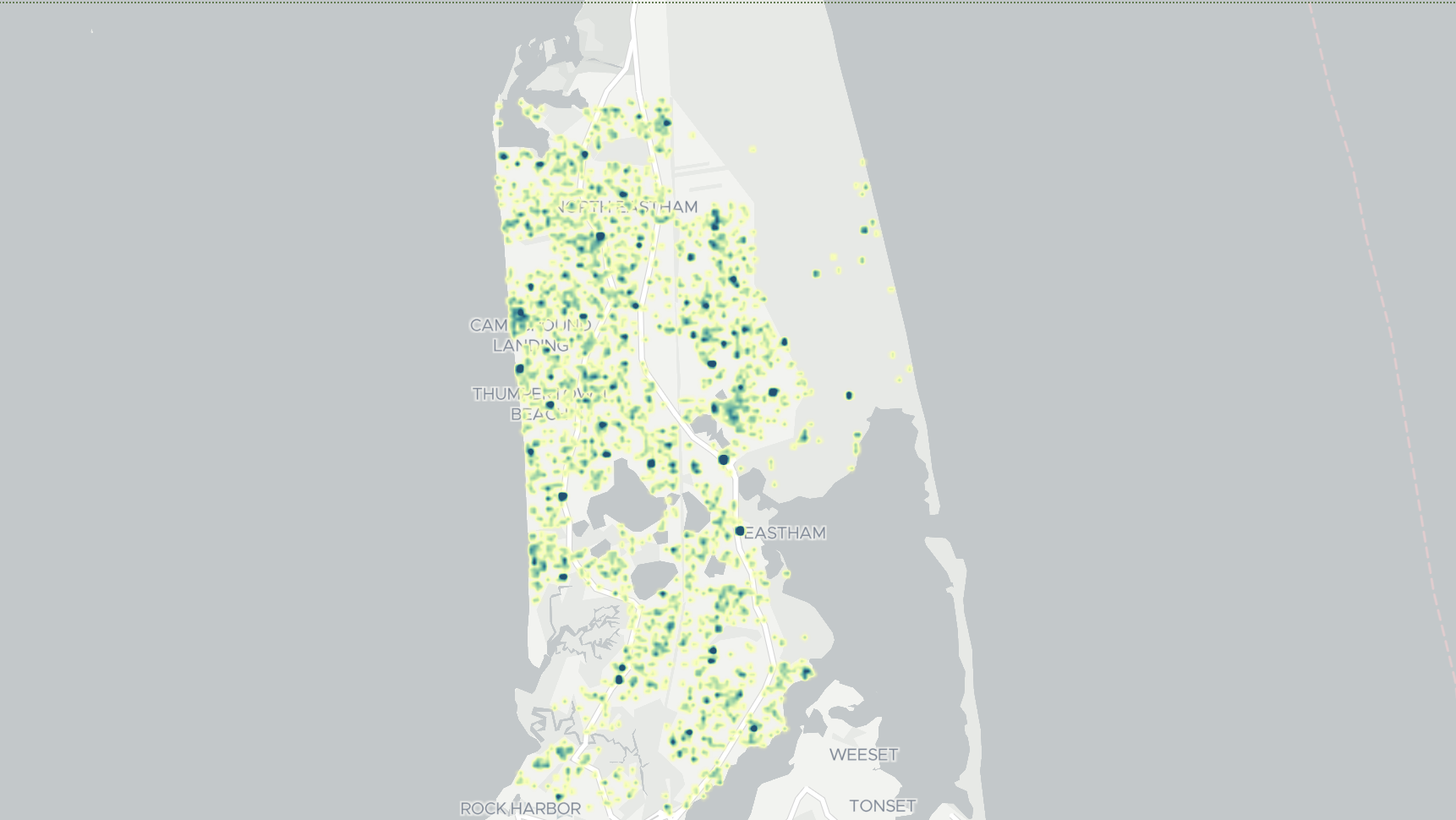
Domestic wells supply drinking water. The distribution and frequency of domestic wells depends on whether a city or town supplies drinking water. Like many areas of the world, cities and towns supply drinking water in more densely populated areas, while wells are used in less densely populated areas.
This pattern is seen in this close-up of eastern Massachusetts. The City of Boston and densely populated surrounding towns are part of a large water district (MWRA). There are few domestic wells in this area or other densely populated areas. Less densely populated areas tend to use domestic wells for drinking water. The pattern repeats on smaller scale. Buildings in city or town centers might use municipal water supplies while those in other areas use wells.
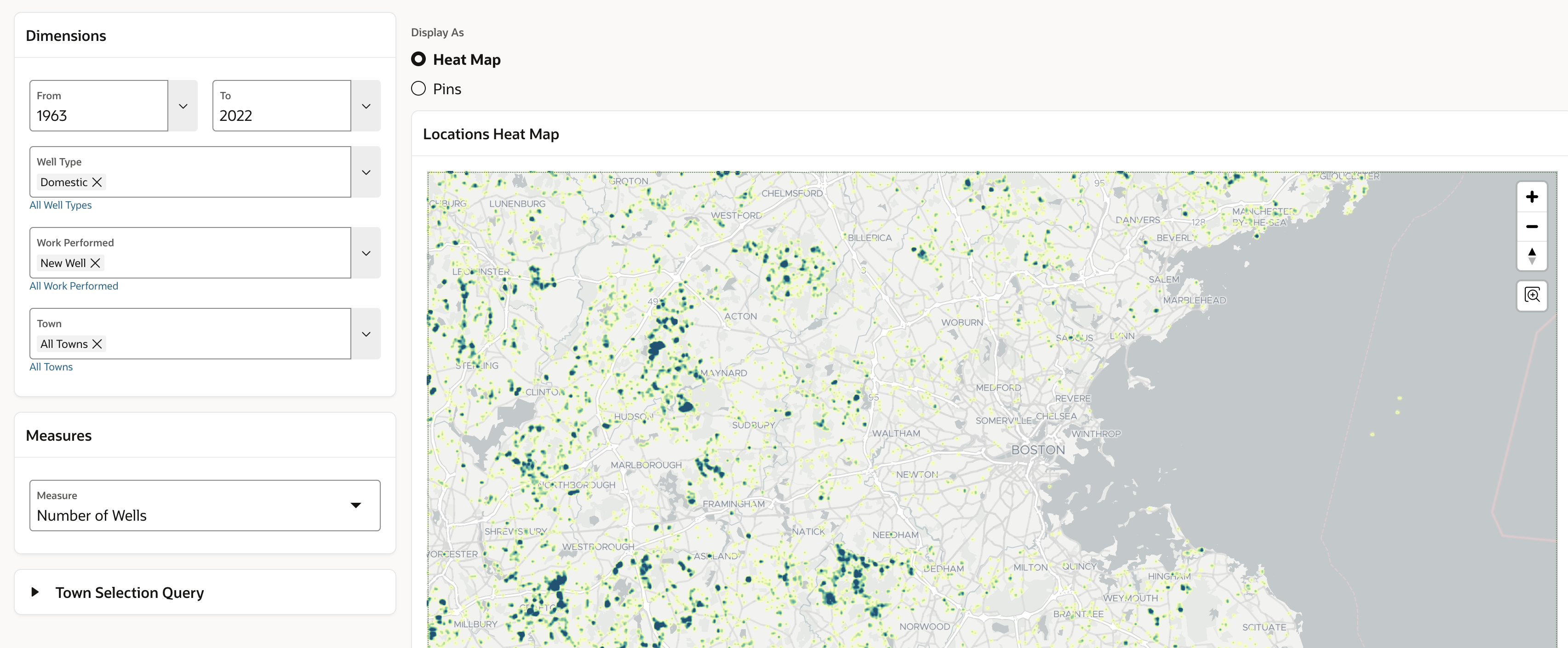
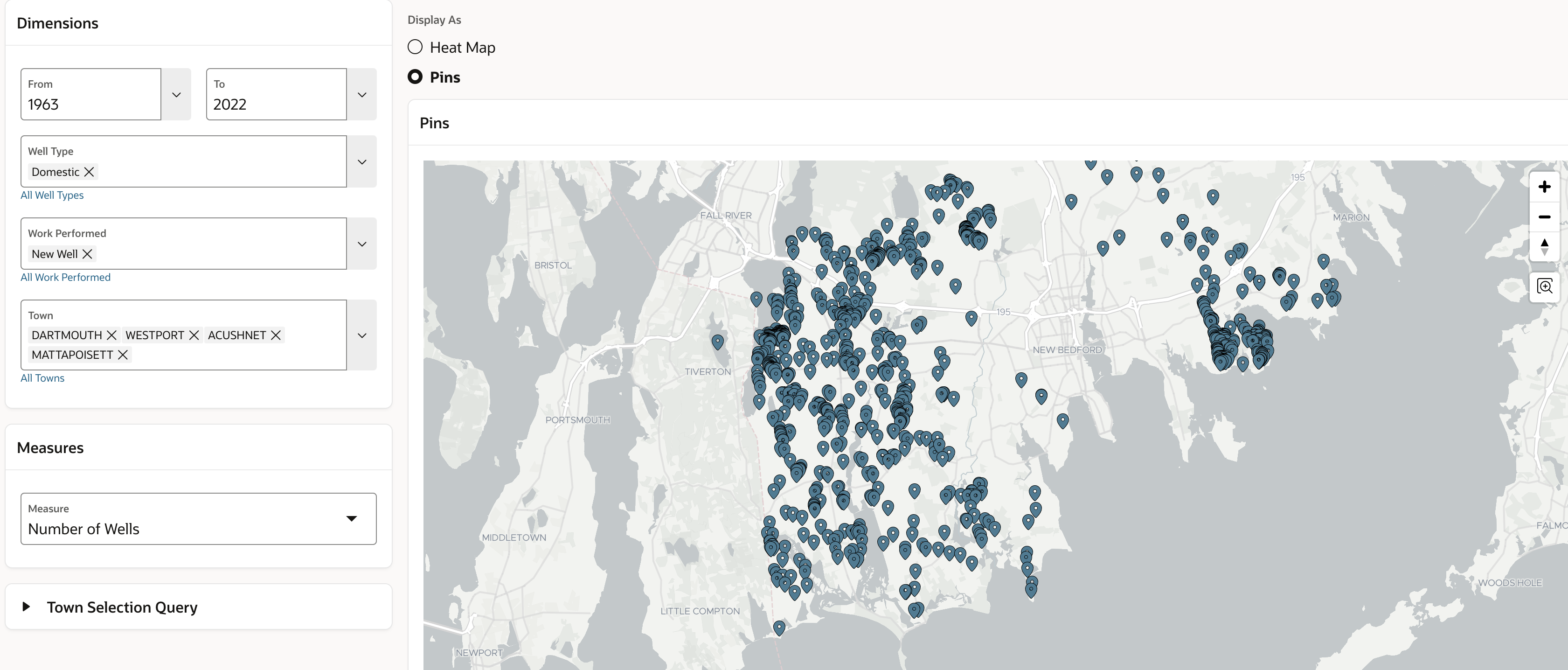
The application allows the user to choose time periods, well types, the type of work performed, and either All Towns or a specific town, as well as the measure. In this close of the South Coast of Massachusetts we see individual domestic well locations.
One Application in Three Query Templates
Let’s start looking at how the application is built.
Each page of this application has two main regions – one for data selection and another for data visualization or reporting. APEX applications are built using pages. Applications may include a global page (page 0) that includes regions and items that can be re-used on other pages, and other pages with page-specific content.
All the items in the Dimensions and Measures regions of this application are on the global page. These regions include a collection of data selection items that are selectively reused on other pages. For example, there are Popup LOV (list of values) items for hierarchies that support either single select or multiple select. Different items support the selection of a range of time periods or a specific time period.
Hierarchy Queries for Popup LOV Items
Each of dimension Popup LOV items using a SQL Query source to select from a hierarchy view.
A hierarchy view includes rows for each hierarchy member of single hierarchy at all levels of aggregation. The hierarchy view includes columns that return properties of the hierarchy member from the underlying table(s) and columns with additional hierarchical properties of the member such as the level name, level key, parent, hierarchical order, and hierarchy depth.
The MEMBER_UNIQUE_NAME column returns the member’s key value. While the structure can vary depending on how the hierarchy is defined, a typical MEMBER_UNIQUE_NAME value takes the form of [level name],&[level_key_value]. For example [WELL_TYPE].&[Irrigation]. The MEMBER_CAPTION column is typically used to return a descriptive value of the hierarchy member, for example ‘Irrigation’. Every hierarchy includes a single grand total value (e.g., [ALL].[ALL]) at the ALL level that represents the grand total of the hierarchy.
This Popup LOV is used to select Well Types.
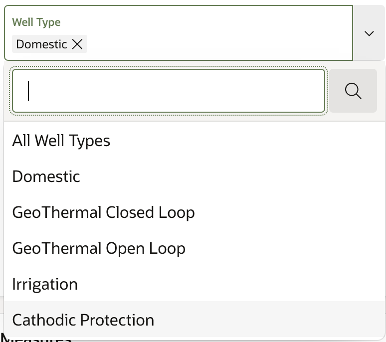
The source of this Popup LOV is a SQL query. The query selects values at the ALL and WELL_TYPE levels.
SELECT
    member_caption d,
    member_unique_name r
FROM
    p8409_well_type
WHERE
    level_name IN ('ALL','WELL_TYPE')
ORDER BY
    hier_order
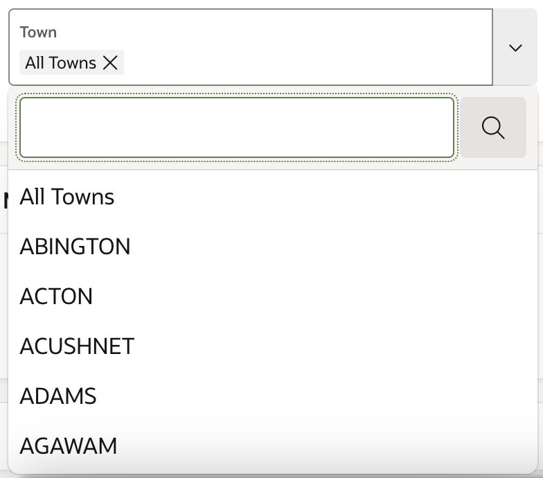
The Popup LOV for each hierarchy uses the same template. For example, this is the query for the Town selection. The queries can, of course, be customized depending on requirements of the application.
The query selects values at the ALL and TOWN levels.
SELECT
    member_caption,
    member_unique_name
FROM
    p8409_town
WHERE
    level_name in ('ALL','TOWN')
ORDER BY
    hier_order
Query for Map Region
The query for the Map region uses a template that selects MEMBER_CAPTION columns (again, the friendly names for hierarchy members), member properties (for example, the LATITUDE and LONGITUDE of a well), and measures. The APEX_STRING.SPLIT table function is used with an IN list to process multiple selections in the Popup LOV hierarchy member selectors.
SELECT
    p8409_town.member_caption AS well_id
    ,p8409_time.member_caption AS time
    ,p8409_well_type.member_caption AS well_type
    ,p8409_work_performed.member_caption AS work_performed
    ,p8409_town.member_caption AS town
    ,p8409_town.latitude AS latitude
    ,p8409_town.longitude AS longitude
    ,NUMBER_OF_WELLS AS my_measure
FROM
    p8409_mass_well_drilling_av
        HIERARCHIES
            (
                p8409_time
                ,p8409_well_type
                ,p8409_work_performed
                ,p8409_town
            )
WHERE
    p8409_time.level_name = 'YEAR'
    AND p8409_time.member_unique_name BETWEEN :P0_FROM AND :P0_TO
    AND p8409_well_type.member_unique_name IN
       (SELECT column_value
        FROM apex_string.split(p_str => :P0_WELL_TYPE_MS,p_sep => ':'))
    AND p8409_work_performed.member_unique_name IN
       (SELECT column_value FROM apex_string.split(p_str => :P0_WORK_PERFORMED_MS,p_sep => ':'))
    AND (:P0_TOWN_MS = '[ALL].[ALL]' OR p8409_town.parent_unique_name IN
        (SELECT column_value FROM apex_string.split(p_str => :P0_TOWN_MS,p_sep => ':')))
    AND p8409_town.level_name = 'WELL_ID'
    AND p8409_town.latitude IS NOT NULL
    AND p8409_town.longitude  IS NOT NULL
This is a typical query of an analytic view, selecting a mix of hierarchical columns, member properties, and measures. Let’s walk through this query from the top down.
The SELECT List
MEMBER_CAPTION columns return the descriptive name of hierarchy members. MEMBER_CAPTION columns are always included in hierarchy views.
SELECT
    p8409_town.member_caption AS well_id
    ,p8409_time.member_caption AS time
    ,p8409_well_type.member_caption AS well_type
    ,p8409_work_performed.member_caption AS work_performed
    ,p8409_town.member_caption AS town
LATITUDE and LONGITUDE are properties of wells. They are needed to plot wells on the map.
    ,p8409_town.latitude AS latitude
    ,p8409_town.longitude AS longitude
NUMBER_OF WELLS is the selected measure. This is a FACT measure in the analytic view, meaning that the measure is mapped and aggregated from the fact table.
,NUMBER_OF_WELLS AS my_measure
The FROM Clause
The query selects from the analytic view P8409_MASS_WELL_DRILLING_AV. P8509 is a prefix I use to keep track of my analytic view objects. I prefer to prefix all objects (attribute dimensions, hierarchies, the analytic view, and sometimes the tables or view) with the same prefix as a grouping mechanism.
FROM
    p8409_mass_well_drilling_av
The HIERARCHIES clause includes hierarchies referenced in the query. Note that joins and GROUP BY are not used in the query. This is because aggregations and joins are included in the definition of the analytic view and hierarchies,
        HIERARCHIES
            (
                p8409_time
                ,p8409_well_type
                ,p8409_work_performed
                ,p8409_town
            )
The WHERE Clause
The application allows the user to choose a range of years. The time hierarchy (P8409_TIME) includes data at DATE_COMPLETED, MONTH and YEAR levels. Because the filter uses BETWEEN, the query filters to the YEAR level so that days or months don’t get mixed in. (BETWEEN will sort VARCHARs alphabetically.)
WHERE
    p8409_time.member_unique_name BETWEEN :P0_FROM AND :P0_TO
    AND p8409_time.level_name = 'YEAR'
Well Type and Work Performed are filtered using an IN list of MEMBER_UNIQUE_NAME columns, which are level key values. Level key values are unique within the hierarchy (across levels) so an additional filter on LEVEL_NAME is not needed.
The application allows multiple selections on some hierarchies. For example, on the Well Type hierarchy.
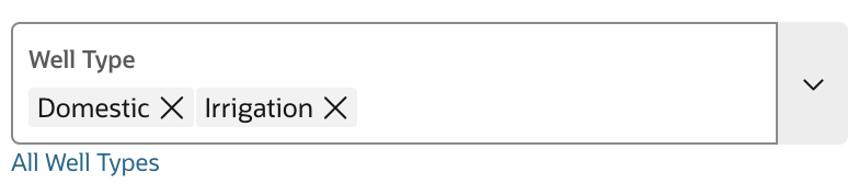
The APEX item is holding the level key values:
[WELL_TYPE].&[Domestic]:[WELL_TYPE].&[Irrigation]
APEX_STRING.SPLIT is a table function that is returns a delimited list of values returned by the APEX item used for the Popup LOV hierarchy member selectors as rows, allowing it to be used in an IN list. (Any query can use APEX_STRING.SPLIT. The application issuing the query does not need to be written in APEX. It’s a great tool.)
     AND p8409_well_type.member_unique_name IN
        (SELECT column_value
         FROM apex_string.split(p_str => :P0_WELL_TYPE_MS,p_sep => ':'))
The town hierarchy (8409_TOWN) includes levels ALL, TOWN and WELL_ID. Each well exists within a town, so there is a hierarchy of WELL_ID CHILD OF TOWN. The map region needs rows for individual wells, with latitude and longitude, so that well locations can be plotted on the map.
The user can choose either All Towns or one or more towns. The filter for the town hierarchy leverages three unique features of the hierarchy view: the ALL member, the PARENT_UNIQUE_NAME column, and the LEVEL_NAME column.
    AND (:P0_TOWN_MS = '[ALL].[ALL]'
         OR p8409_town.parent_unique_name IN
          (SELECT column_value
             FROM apex_string.split(p_str => :P0_TOWN_MS,p_sep => ':')))
    AND p8409_town.level_name = 'WELL_ID'
If the user chooses All Towns (where the key value is [ALL].[ALL]) the filter evaluates to
('[ALL].[ALL]' = '[ALL].[ALL]' OR p8409_town.parent_unique_name = '[ALL].[ALL]')
This will result in the selection of all wells.
If one or more towns are selected, for example EASTHAM the filter evaluates to.
('[TOWN].[EASTHAM]' = '[ALL].[ALL]'
  OR p8409_town.parent_unique_name IN ('[TOWN].[EASTHAM]')
This will result in the selection of wells within the town of Eastham.
The filter P8409_TOWN.LEVEL_NAME = ‘WELL_ID’ is needed for the All Towns case.. Without it rows at the ALL, TOWN and WELL_ID levels would be returned.
This might seem a bit complicated, but it’s really not. Once you take a look at how hierarchies work it will become clear. The Oracle LiveSQL Tutorial Querying Analytic Views – Getting Started is a great place to learn about querying analytic views.
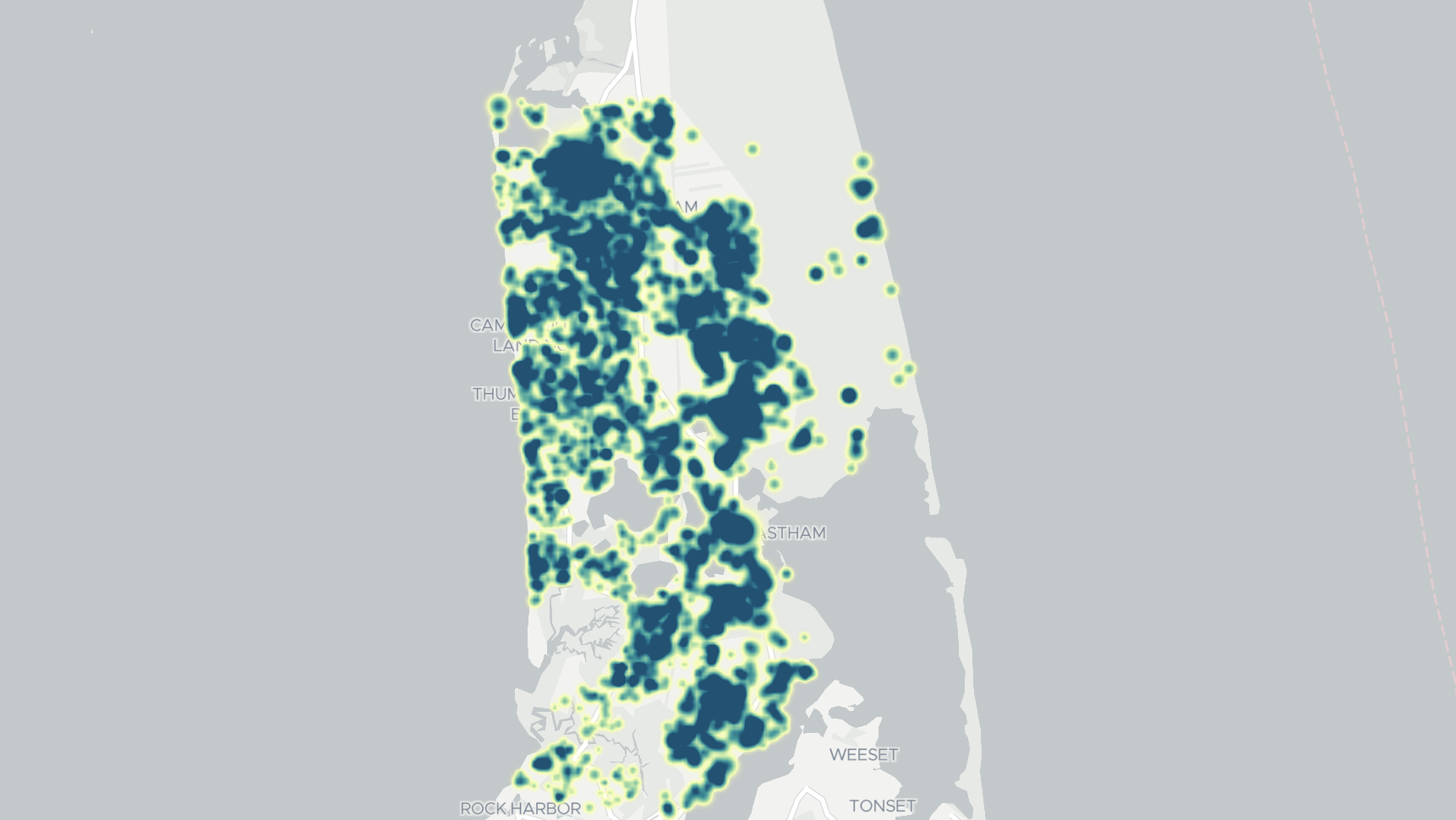
In the analytic view, the value for NUMBER_OF_WELLS is always one (one well per row). The heat map will simply display the concentration of wells.
Changing the Measure Selection
To display the average well depth, the user chooses the Avg Total Depth measure. The query selects that measure using the same query template as was used with Number of Wells. The selected measure is substituted using the bind variable of measure Popup LOV item (PO_MEASURE).
It really doesn’t get any easier than that.
SELECT
    p8409_town.member_caption AS well_id
    ,p8409_time.member_caption AS time
    ,p8409_well_type.member_caption AS well_type
    ,p8409_work_performed.member_caption AS work_performed
    ,p8409_town.member_caption AS town
    ,p8409_town.latitude AS latitude
    ,p8409_town.longitude AS longitude
    ,AVG_TOTAL_DEPTH AS my_measure
FROM
    p8409_mass_well_drilling_av
        HIERARCHIES
            (
                p8409_time
                ,p8409_well_type
                ,p8409_work_performed
                ,p8409_town
            )
WHERE
    p8409_time.level_name = 'YEAR'
    AND p8409_time.member_unique_name BETWEEN :P0_FROM AND :P0_TO
    AND p8409_well_type.member_unique_name IN
        (SELECT column_value FROM apex_string.split(p_str => :P0_WELL_TYPE_MS,p_sep => ':'))
    AND p8409_work_performed.member_unique_name IN
        (SELECT column_value FROM apex_string.split(p_str => :P0_WORK_PERFORMED_MS,p_sep => ':'))
    AND (:P0_TOWN_MS = '[ALL].[ALL]' OR p8409_town.parent_unique_name IN
        (SELECT column_value FROM apex_string.split(p_str => :P0_TOWN_MS,p_sep => ':')))
    AND p8409_town.level_name = 'WELL_ID'
    AND p8409_town.latitude IS NOT NULL
    AND p8409_town.longitude IS NOT NULL
Here we can observe variability in total well depth.
How Deep are Domestic Wells?
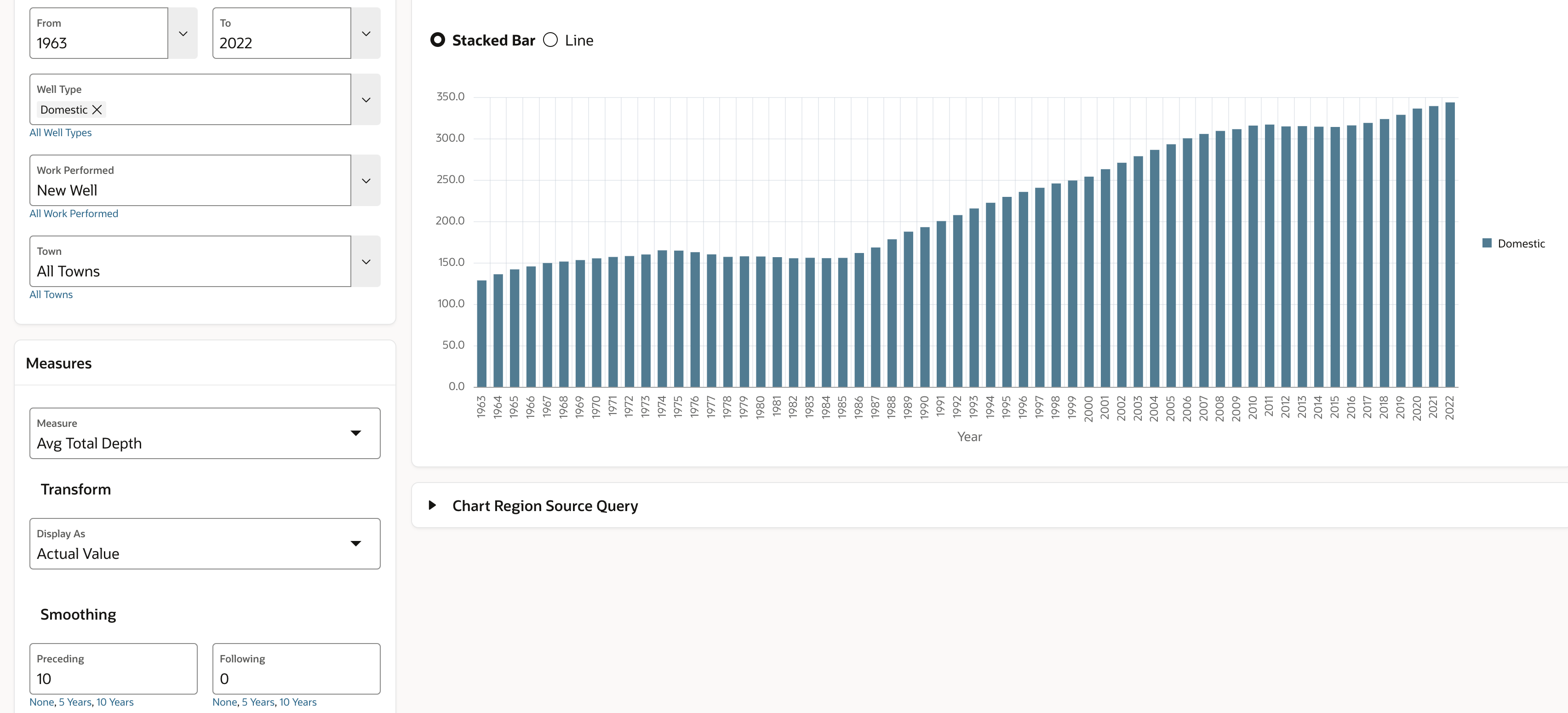
How deep are domestic wells? It depends on where the well is, and when the well was drilled. New domestic wells in Massachusetts have averaged about 350 feet over the last 5 years.
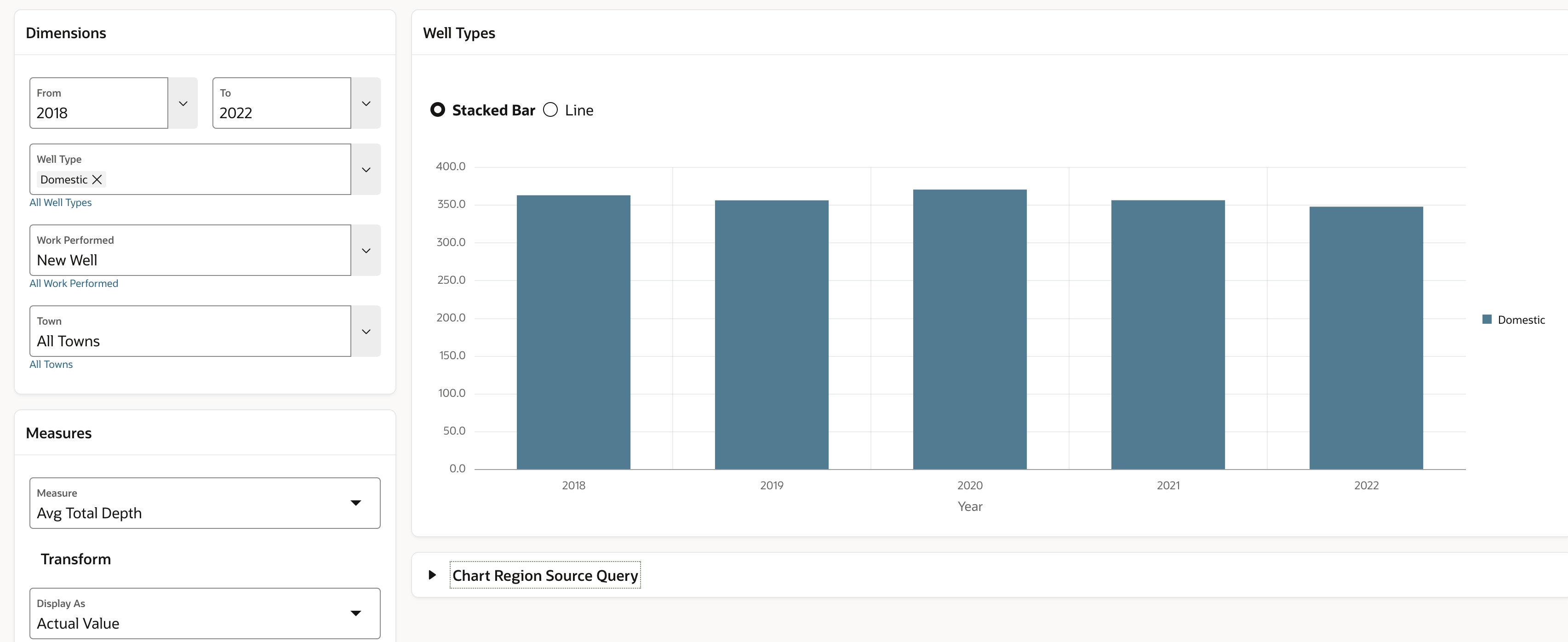
Notice the Measures selection for this page include parameters for transforming the measure. This page supports displaying the selected measure as the Actual Value, the Change Prior Period and the Percent Change Prior Period. User can also choose to smooth the data using a moving average.
Unlike Western U.S. states, water is relatively plentiful in the Northeastern U.S. Even so, wells have been drilled deeper over time. If we extend the time selection from 1963 to 2022 and use a 10-year moving average to smooth the data, we can see a steady increase in average domestic well depth.
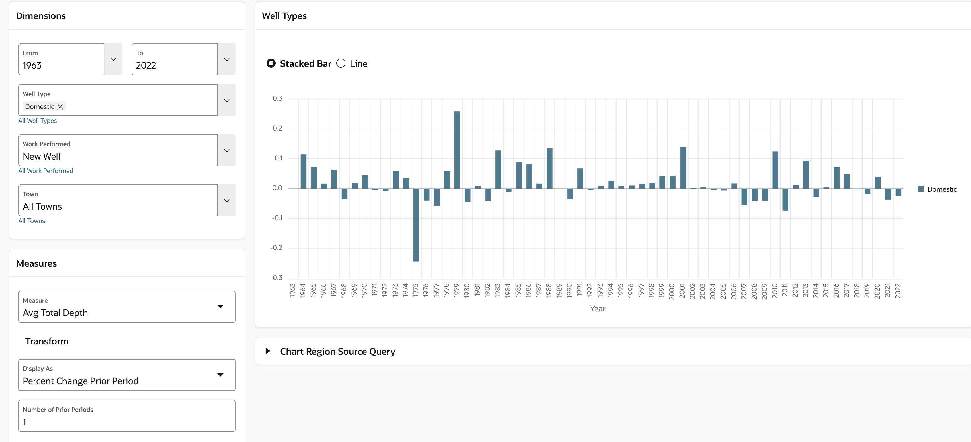
We can also view the year-over-year percent change in average well depth.
The year over year change looks rather ‘noisy’, so we can smooth it using a 5-year moving average. The trend becomes more clear.
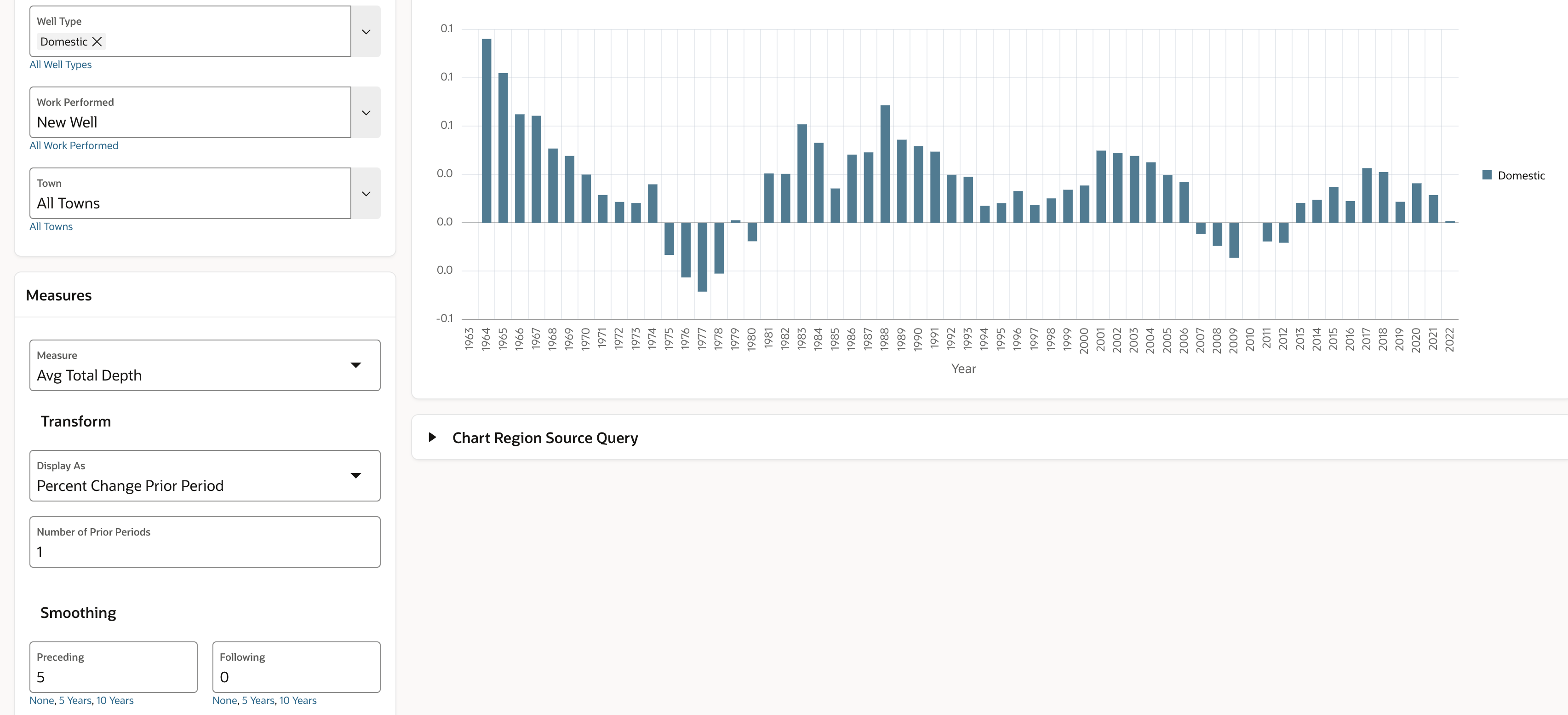
5 year moving average, year over year percent change in total well depth for all cities and towns.
What does it take to produce the query for a 5-year Moving Average of the Percent Change of a Prior Period of an Average Well Depth at aggregate levels of each of the hierarchies?
If you are using an Analytic View, it’s easy. There are two implementation paths:
- Define calculated measures in the analytic view and select them just like any other measure using a query like the one used with the map.
- Define the calculated measure on the fly in the select statement.
The calculation expression is the same with either approach, it’s just a difference of where the calculation is defined. The expression for the 5-year Moving Average of the Percent Change Prior Year is:
AVG(
      LAG_DIFF(AVG_TOTAL_DEPTH) OVER (HIERARCHY p8409_time OFFSET 1)
   OVER (HIERARCHY p8409_time BETWEEN 10 PRECEDING AND 0 FOLLOWING WITHIN LEVEL)
This expression nests the change from prior period (LAG_DIFF) within a moving average (AVG).
Note that analytic view expression references elements of the model such as hierarchies and levels rather than columns. Unlike queries that select from tables using the LAG window function, the analytic view expression is the same for every query. This is of tremendous benefit to the APEX application developer.
The application allows the user to apply transformations to each base measure. If each permutation was defined as a calculated measure in the Analytic View, 36 calculated measures would be needed (4 base measures * 3 time series calculation * 3 predefined smoothing periods). And that doesn’t account for allowing the user to choose the number of prior periods.
Alternatively, calculations can be expressed on the fly. This approach also allows the user to choose the number of smoothing periods and the prior period offset (the number of prior periods). This is a case where the APEX developer has an advantage over a business intelligence tool that can only select from measures in the analytic view. Because the APEX developer has complete control of the SQL, they can create calculated measures on the fly.
This application uses the on-the-fly approach.
This form of the query uses the USING clause and ADD MEASURES. Otherwise, it’s the same as the query used with the map region. As many calculation measures as needed can be included in ADD MEASURES. The expression is the same as the example above.
SELECT
    p8409_town.member_caption AS town
    ,p8409_time.year
    ,p8409_well_type.member_caption as well_type
    ,p8409_work_performed.member_caption as work_performed
    ,measure
  FROM ANALYTIC VIEW (
    USING p8409_mass_well_drilling_av
        HIERARCHIES
            (
                p8409_time
                ,p8409_well_type
                ,p8409_work_performed
                ,p8409_town
            )
        ADD MEASURES (
            measure AS (AVG(
                         LAG_DIFF_PERCENT(AVG_TOTAL_DEPTH) OVER (HIERARCHY p8409_time OFFSET 1)
                         ) OVER (HIERARCHY p8409_time BETWEEN 5 PRECEDING AND 0 FOLLOWING WITHIN LEVEL))
            )
        )
WHERE
    p8409_time.level_name = 'YEAR'
    AND p8409_time.member_unique_name BETWEEN :P0_FROM AND :P0_TO
    AND p8409_well_type.member_unique_name IN
        (SELECT column_value FROM apex_string.split(p_str => :P0_WELL_TYPE_MS,p_sep => ':'))
    AND p8409_work_performed.member_unique_name = :P0_WORK_PERFORMED
    AND p8409_town.member_unique_name = :P0_TOWN
ORDER BY
    p8409_time.hier_order
Well Enhancements
It’s reasonable to think that wells are being drilled deeper for improved production. On the Work Performed page we can look at wells that have been enhanced by deepening and hydrofracturing, and we see that there is a concentration of domestic well enhancements in east-central Massachusetts.
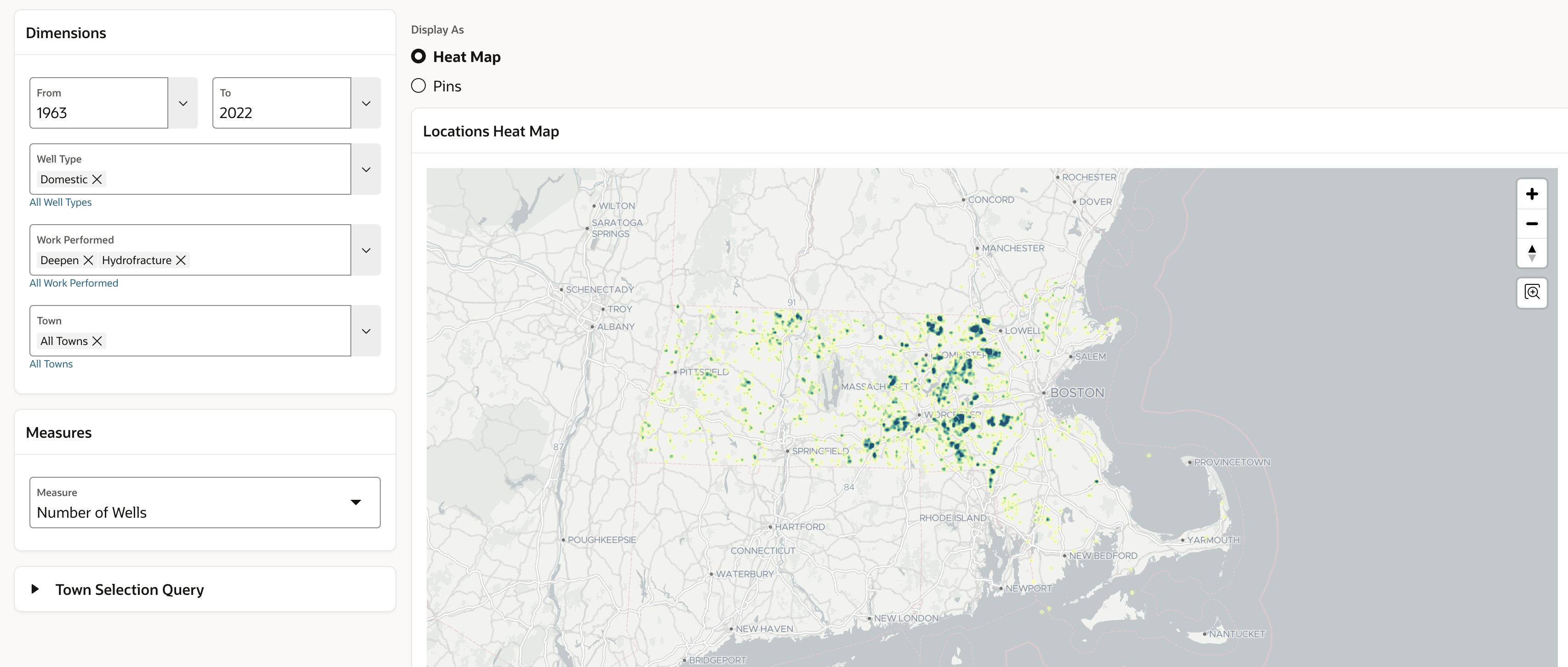
We can get a good sense of well enhancement trends by looking at a 5-year moving average of wells that have been deepened and hydro-fractured.
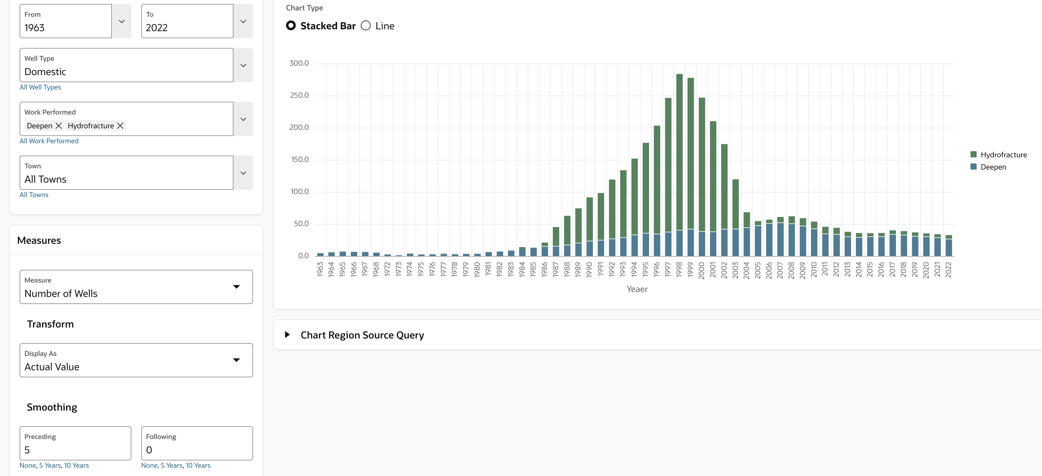
5-year moving average of enhanced domestic wells
What does the query look like? It’s the same template with a different measure in ADD MEASURES.
SELECT
        p8409_town.member_caption AS well_id
        ,p8409_time.year
        ,p8409_well_type.member_caption as well_type
        ,p8409_work_performed.member_caption as work_performed
        ,p8409_town.town AS town
        ,measure
  FROM ANALYTIC VIEW (
    USING p8409_mass_well_drilling_av
        HIERARCHIES
            (
                p8409_time
                ,p8409_well_type
                ,p8409_work_performed
                ,p8409_town
            )
        ADD MEASURES (
            measure AS (AVG(
                            NUMBER_OF_WELLS
                         ) OVER (HIERARCHY p8409_time BETWEEN 5 PRECEDING AND 0 FOLLOWING WITHIN LEVEL))
            )
        )
WHERE
    p8409_time.level_name = 'YEAR'
    AND p8409_time.member_unique_name BETWEEN :P0_FROM AND :P0_TO
    AND p8409_well_type.member_unique_name = :P0_WELL_TYPE
    AND p8409_work_performed.member_unique_name IN (SELECT column_value FROM apex_string.split(p_str => :P0_WORK_PERFORMED_MS,p_sep => ':'))
    AND p8409_town.member_unique_name = :P0_TOWN
ORDER BY
    p8409_time.hier_order
Distribution Patterns by Well Type
There are different distribution patterns for different well types. Irrigation wells show the opposite pattern from domestic wells, with the heaviest concentration in Eastern Massachusetts.
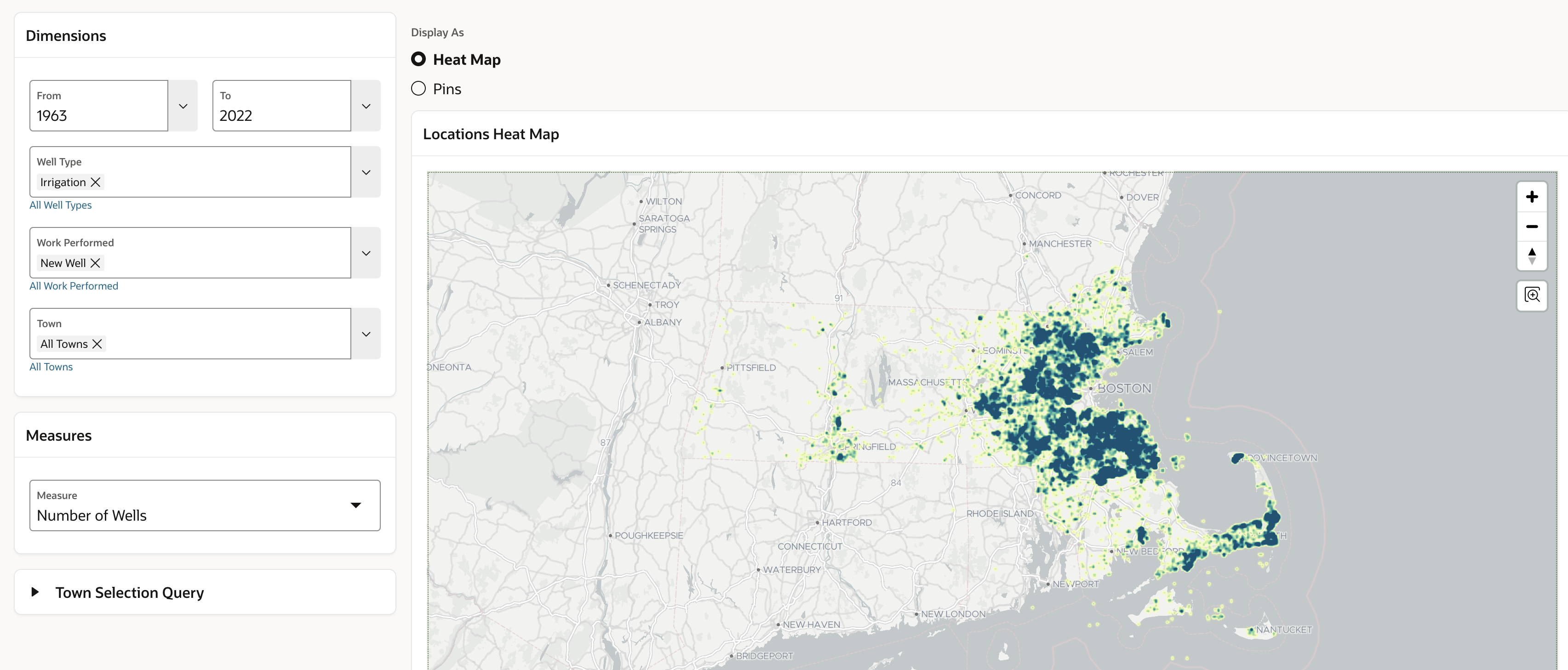
A few possibilities are that:
- Eastern Massachusetts and Cape Cod tend to be more wealthy than other areas and people with nice houses like nice landscaping, and perhaps they like to irrigate their landscaping.
- There are often restrictions on the amount of water used during the hot summer months, just when irrigation is needed. Perhaps wells are a good solution.
- People with domestic wells can also using water for landscaping (providing that the well is productive enough), so it is less likely they would have a well dedicated for irrigation.
This data set doesn’t really answer those questions, but it does point out some interesting distribution patterns that might prompt further investigation.
What does the query look like for this query? Just like the others. 🙂
SELECT
        p8409_town.member_caption AS well_id
        ,p8409_time.member_caption AS time
        ,p8409_well_type.member_caption AS well_type
        ,p8409_work_performed.member_caption AS work_performed
        ,p8409_town.member_caption AS town
        ,p8409_town.latitude AS latitude
        ,p8409_town.longitude AS longitude
        ,NUMBER_OF_WELLS AS my_measure
FROM
        p8409_mass_well_drilling_av
                HIERARCHIES
                        (
                                p8409_time
                                ,p8409_well_type
                                ,p8409_work_performed
                                ,p8409_town
                        )
WHERE
        p8409_time.level_name = 'YEAR'
        AND p8409_time.member_unique_name BETWEEN :P0_FROM AND :P0_TO
        AND p8409_well_type.member_unique_name IN
                (SELECT column_value FROM apex_string.split(p_str => :P0_WELL_TYPE_MS,p_sep => ':'))
        AND p8409_work_performed.member_unique_name IN
                (SELECT column_value FROM apex_string.split(p_str => :P0_WORK_PERFORMED_MS,p_sep => ':'))
        AND (:P0_TOWN_MS = '[ALL].[ALL]' OR p8409_town.parent_unique_name IN
                (SELECT column_value FROM apex_string.split(p_str => :P0_TOWN_MS,p_sep => ':')))
        AND p8409_town.level_name = 'WELL_ID'
        AND p8409_town.latitude IS NOT NULL
        AND p8409_town.longitude    IS NOT NULL
Distribution of New Irrigation Wells over Time
The data does tell us when the irrigation wells were drilled. The following chart examines new irrigation wells from 1980 to 2022.
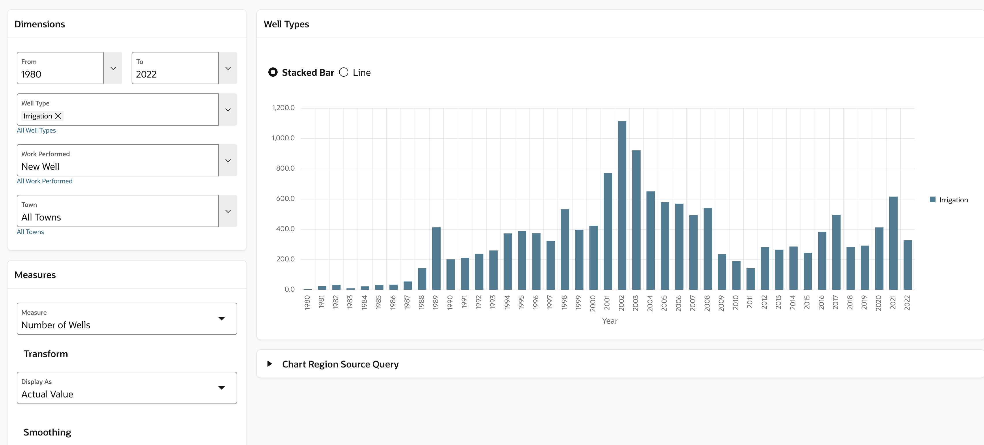
A reasonable hypothesis is that people spend more money on nice homes and landscaping when they are making more money. Here we see a correlation with the rise of high-tech and biotechnology in Greater Boston with landscape well drilling. We see a steep rise leading up to the dot.com bubble (2000) and a steep fall off after the bubble popped. We see another steep drop after the financial crisis of 2008, and a slow recovery afterward. Perhaps the spike in 2020 and 2021 was driven by people staying home during COVID and tending their gardens.
A chart with the change from prior period 2 year moving average helps bring this into focus. The peaks and valleys does resemble stock market indices. Again, the data neither proves of disproves the hypothesis. You decide. It does help us ask new questions.
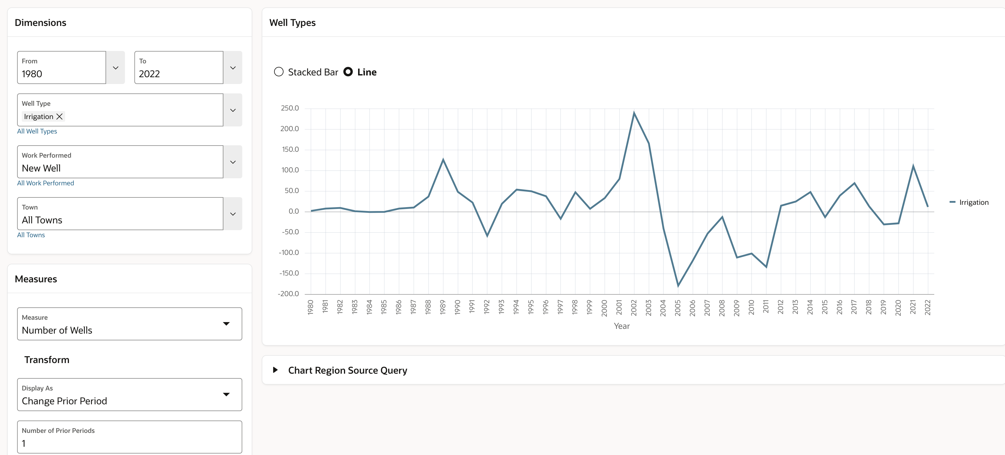
And what does the query look like? Ok, one more time.
SELECT
    p8409_town.member_caption AS town
    ,p8409_time.year
    ,p8409_well_type.member_caption as well_type
    ,p8409_work_performed.member_caption as work_performed
    ,measure
  FROM ANALYTIC VIEW (
    USING p8409_mass_well_drilling_av
        HIERARCHIES
            (
                p8409_time
                ,p8409_well_type
                ,p8409_work_performed
                ,p8409_town
            )
        ADD MEASURES (
            measure AS (AVG(
                            LAG_DIFF(NUMBER_OF_WELLS) OVER (HIERARCHY p8409_time OFFSET 1)
                         ) OVER (HIERARCHY p8409_time BETWEEN 2 PRECEDING AND 0 FOLLOWING WITHIN LEVEL))
            )
        )
WHERE
    p8409_time.level_name = 'YEAR'
    AND p8409_time.member_unique_name BETWEEN :P0_FROM AND :P0_TO
    AND p8409_well_type.member_unique_name IN
        (SELECT column_value FROM apex_string.split(p_str => :P0_WELL_TYPE_MS,p_sep => ':'))
    AND p8409_work_performed.member_unique_name = :P0_WORK_PERFORMED
    AND p8409_town.member_unique_name = :P0_TOWN
ORDER BY
    p8409_time.hier_order
Summary
When you first started reading this post you might have been wondering ‘why write a post using well drilling data from MassachusettS?’. What could possibility be interesting about that? And what how could Oracle APEX be used to help understand this data?
I hope you agree that there are some interesting observations have been made, and that building an application such as this is actually very easy. No, it’s not a replacement for a full featured business intelligence tool, but APEX and Analytic Views are a very powerful combination and a great platform for certain types of applications.
And don’t forget, if you are using the Oracle Database you already have everything you need to build an application like this.
Take a Look for Yourself
Feel free to look at the data using the Massachusetts Well Drilling application. This application is running on Oracle Autonomous.
Learn More
Learn about Oracle Autonomous Database. Did you know that there is Autonomous Database Data Warehouse and Autonomous Database for Application Express? Did you know that Autonomous Database is available with Always Free? You could build an application like this one for free!
Get started with Oracle Application Express today at apex.oracle.com. This is a great place for beginners and experienced users.
Learn about creating and querying analytic views using SQL at Oracle Live SQL. There are over a dozen tutorials for analytic views.