Using Jupyter on OCI Data Science to analyze HPC results

High-performance computing (HPC) on Oracle Cloud Infrastructure (OCI) accelerates the delivery of complex, time-consuming numerical simulations by running that simulation’s many compute tasks in parallel across the HPC cluster’s multiple compute nodes. Those compute nodes provide a reservoir of CPUs or GPUs, memory, and network bandwidth that allows you to swiftly complete a parallelized simulation too time-consuming for serial running. Typical use cases include physical simulations for product design, clinical research, financial modeling, oil and gas reservoir modeling, and more.

Often, you’re also performing multiple HPC calculations so that key design parameters can be optimized. Examples include selecting an airplane’s shape so that safety and performance are maximized or the design of a sophisticated financial instrument so that risk and revenue are properly balanced.

Optimizing those design parameters requires inspecting the output generated by those many HPC simulations. This blog post shows how easily you can use OCI Data Science, which provides compute, memory, and a Jupyter server with the usual Python libraries (NumPy, pandas, matplotlib, and so on) preinstalled so you can quickly develop custom Python code to visualize your HPC output. OCI Data Science also helps optimize your simulations’ design settings.

This blog post walks you through the deployment of an HPC cluster on OCI, the installation of a computational fluid dynamics (CFD) code on that cluster, the parallel run of that code across the cluster, and then using Data Science to visualize the HPC output. We briefly summarize the key steps, but for more details, see this GitLab demo.

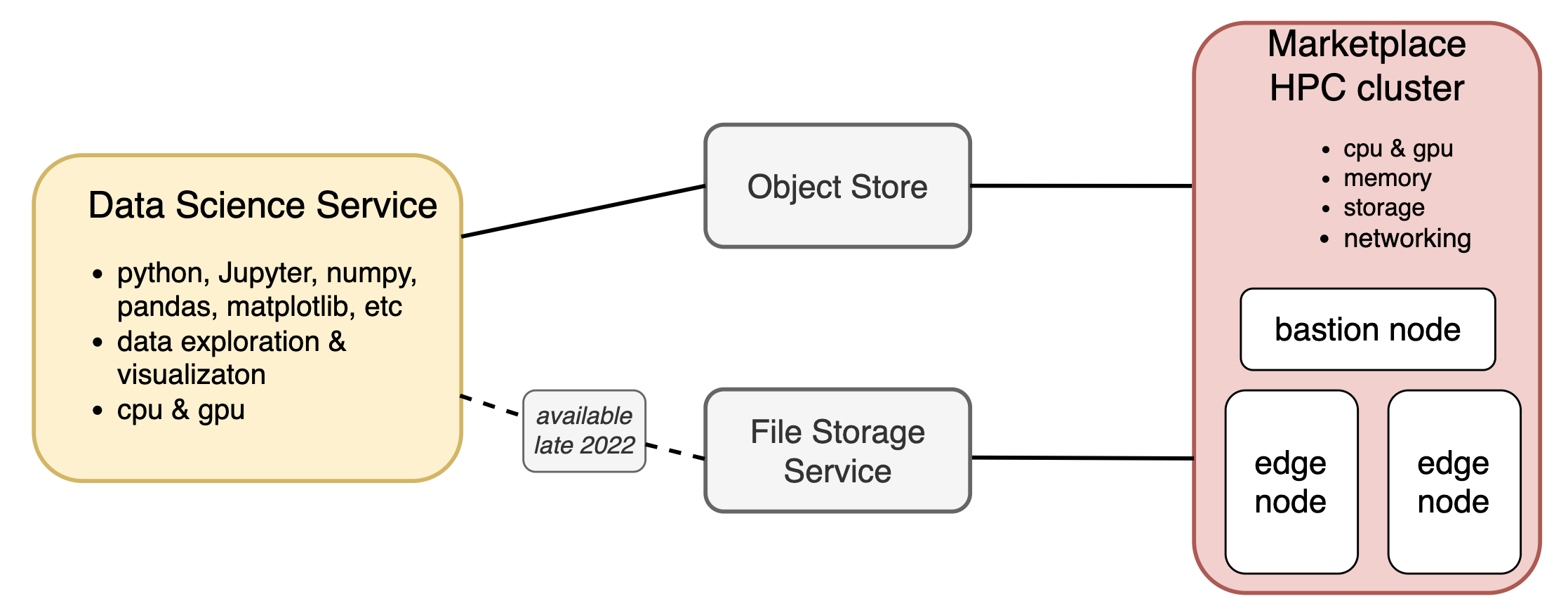
^{Figure 1. Cloud architecture for HPC and Data Science}

Deploy an HPC cluster

Figure 1 shows the cloud architecture used in this example. In the Oracle Cloud Marketplace, select HPC Cluster Stack to create an HPC cluster. Select the number of compute nodes, their shape, and their storage, and give the new cluster a name. This example builds the smallest possible HPC cluster, composed of two bare metal compute nodes using the BM.HPC2.36 shape, which provides 384 GB of memory and 36 compute cores on each node.

Clicking the Create button runs an OCI-provided Terraform script that deploys an HPC stack composed of two compute nodes and a bastion instance, with all instances having all the standard HPC libraries preinstalled. You can also tailor the Terraform script further so that any other libraries and custom settings are also present at subsequent deployments. Deploying an HPC cluster within OCI is easy, and tailoring that cluster to a specific use case is straightforward.

Next, SSH into the bastion node, which serves as the cluster’s front door and is where the HPC job is deployed. This example runs the FARGO3D code on the HPC cluster. FARGO3D is a CFD code that solves the differential equations that govern how flowing fluids evolve. FARGO3D is used for astrophysics research, which is irrelevant to most users of OCI’s HPC. Nevertheless, FARGO3D is easy to install, run, and visualize its output, and why we’re using it in our example. FARGO3D was developed to study the formation and evolution of recently formed planets orbiting within the circumstellar disk of gas and solids from which they formed. Our example simulates the mutual coevolution of a recently formed planet while its gravity disturbs the dusty gas disk that also birthed it.

Install and set up FARGO3D

Running the HPC job that performs the parallel run of FARGO3D also requires a simple bash script posted at a Github repo, and this walkthrough assumes that you clone that repo to your bastion node from the following source:

git clone git@github.com:oracle-nace-dsai/fargo3d-demo.git
cd fargo3d-demo

Then download and unpack FARGO3D:

wget http://fargo.in2p3.fr/downloads/fargo3d-1.3.tar.gz
tar -xvf fargo3d-1.3.tar.gz
cd fargo3d-1.3

Then compile FARGO3D for a parallel run with the following command:

make SETUP=fargo PARALLEL=1 GPU=0

The FARGO3D code comes with a file containing the initial conditions for the disk-planet system described, but to make our HPC simulation more challenging, replace the FARGO3D-provided initial conditions with a modified version that samples the disk’s CFD grid 16 times more finely and extends the simulation’s timewise duration by five times. Overwrite the original fargo.par file with the modified version:

cp ../fargo_big.par setups/fargo/fargo.par

The slurm workload manager is used to run FARGO3D in parallel across the cluster’s compute nodes. So, copy the slurm deployment script to the working directory and inspect:

cp ../MY_SLURM_JOB .
cat MY_SLURM_JOB

This command displays the following result:

#!/bin/bash
module load mpi/openmpi/openmpi-4.0.3rc4
time mpirun ./fargo3d -k ./setups/fargo/fargo.par

When this deployment script is processed, it first loads an openmpi module that uses the Message Passing Interface (MPI) library to run FARGO3D’s various code tasks in parallel. The script then tells mpirun to run FARGO3D in parallel using the now-modified initial conditions, with this job’s runtime also being tracked.

Run the slurm job

This experiment’s FARGO3D job is submitted to slurm with the following command:

sbatch --job-name=fargo3d --nodes=2 --ntasks-per-node=32 --cpus-per-task=1 --exclusive MY_SLURM_JOB

This command tells slurm to run 32 parallel tasks on each of this cluster’s compute nodes, with one CPU dedicated to each task. This slurm job completes in 30 minutes on this small HPC cluster, and inspection of OCI’s cloud-compute cost tells us that this 30-minute-long HPC experiment accrued a $2.80 cloud bill.

Next, check how process times and compute costs scale by rerunning this example with --nodes=1 and --ntasks-per-node=1, which instructs slurm to run this job using only 1 CPU on a single compute node. That single-threaded FARGO3D job completes in 19 hours, which costs $3.05 if the run instead occurred on a typical OCI instance of shape VM.Standard2.4. So, if lengthy run times are impacting your project’s time to deliver, consider migrating your parallelizable workloads to HPC, where run times can be shorted dramatically with no incremental compute costs.

Visualizing HPC output with OCI Data Science

Deploy and configure a Data Science instance to communicate with the HPC cluster, and consult this document for the required steps. This experiment originally intended to use OCI’s File Storage System to manage the HPC cluster’s output. The DS-FSS connectivity isn’t available for a few months, so instead use OCI’s command line interface (OCI CLI) to manually copy the HPC output to an OCI Object Storage bucket where the Data Science instance can see it. See also Figure 1 and these more detailed instructions.

Then navigate to the Data Science instance’s Jupyter server, where you can develop custom Python code to read, analyze, and visualize the HPC output inside this Jupyter notebook, with Figures 2–4 displaying highlights from that analysis.

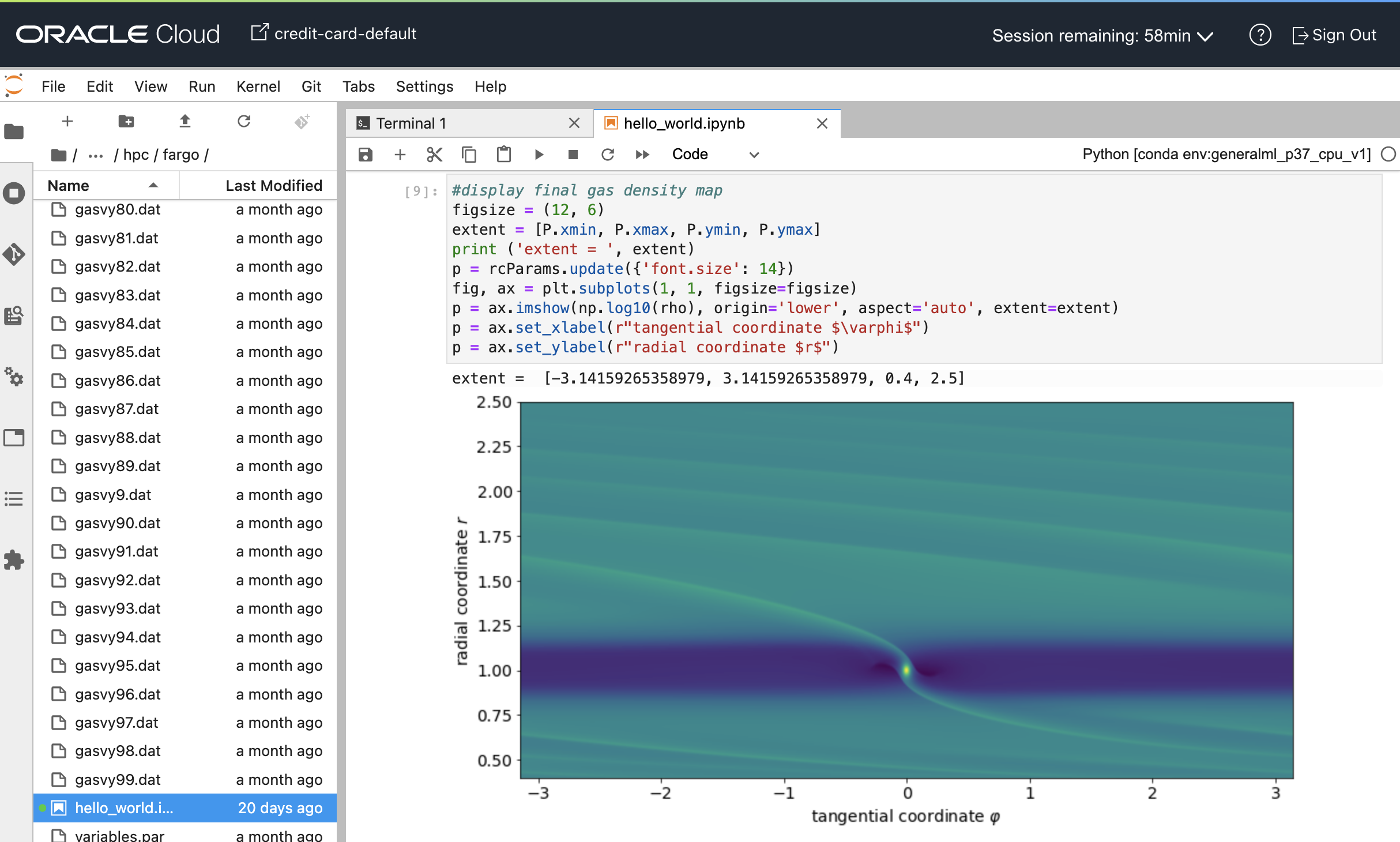
^{Figure 2. Example notebook that reads and visualizes output generated by FARGO3D simulation.}

OCI Data Science provides a Jupyter notebook where you can prototype and develop custom Python code to analyze and visualize HPC output. The notebook shown in Figure 2 displays the final state of the FARGO3D simulation of a Jupiter-mass planet orbiting within a circumstellar disk. That FARGO3D simulation uses a polar (r, j) coordinate grid to track the mutual evolution of the disk-planet system. The heatmap in Figure 2 shows the gas disk’s density displayed with disk radius r increasing upwards and disk azimuth j to the right.

This visualization scheme ‘unwraps’ the disk and reprojects it onto a rectangular grid. The planet, which has its own circumplanetary gas disk, is at the bright spot in the lower middle, and the horizontal dark band is an annulus of low-density gas that was depleted by the planet’s gravitational perturbations of the disk. Tilted density bands are spiral density waves that the planet also excites within the disk.

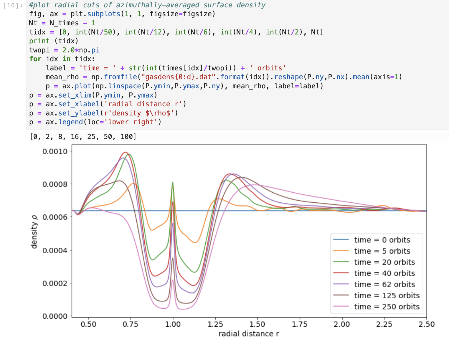
^{Figure 3. Code block plotting simulated gas disk’s density versus radial distance at various simulation times}

Figure 3 shows radial profiles of the disk’s azimuthally averaged density r at various simulation times. The planet’s gravitational perturbations open an annular gap in the gas disk concentric with the planet’s orbit at r=1. The density peak at r=1 is due to residual disk gas that persists along the planet’s orbit.

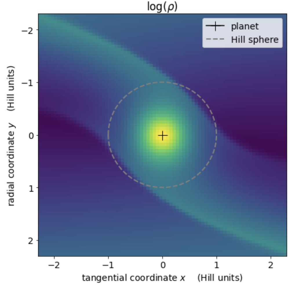
^{Figure 4. Heatmap of the circumplanetary disk}

The Figure 4 heatmap zooms in on the immediate vicinity of planet that resides at the + and is surrounded by a circumplanetary disk of gas and solids that is supplied by two streams of circumstellar matter that go into orbit about the planet when inside that planet’s Hill radius, which is where the planet’s gravity dominates over stellar gravity.

Recommendations

When the serial run of your use case’s numerical simulations is excessive and slows your solution’s delivery, investigate whether a parallel run of that code is possible. If so, get those parallelized simulations processed much more swiftly using Oracle Cloud Infrastructure’s HPC offering, which this example shows to be cost-effective. If you also need custom code to investigate the HPC output, consider developing your visualizations using Oracle’s Data Science service using the simple cloud architecture shown in Figure 1.

For more information about the topics mentioned in this blog post, see the following resources:

• Oracle Cloud Infrastructure

• High-performance computing

• Computational fluid dynamics

• FARGO3D

• Message Passing Interface (MPI)

• OCI Command Line Interface (CLI)

• OCI Data Science

• slurm